Signal-to-Noise Ratio

Imagine developing a song recognition application. The software’s goal is to recognize a song even when it’s played in a noisy environment, similar to Shazam. To achieve this, you want to enhance the audio quality by reducing the noise and evaluating the improvement using the Signal-to-Noise Ratio (SNR).

In this example, we will demonstrate how to generate a clean signal, add varying levels of noise to simulate the noisy recording, use FFT for noise reduction, and then evaluate the quality of the reconstructed audio using SNR.

Import necessary libraries

from typing import Tuple

import matplotlib.animation as animation
import matplotlib.pyplot as plt
import numpy as np
import torch
from torchmetrics.audio import SignalNoiseRatio

# Set seed for reproducibility
torch.manual_seed(42)
np.random.seed(42)

Generate a clean signal (simulating a high-quality recording)

def generate_clean_signal(length: int = 1000) -> Tuple[np.ndarray, np.ndarray]:
    """Generate a clean signal (sine wave)"""
    t = np.linspace(0, 1, length)
    signal = np.sin(2 * np.pi * 10 * t)  # 10 Hz sine wave, representing the clean recording
    return t, signal

Add Gaussian noise to the signal to simulate the noisy environment

def add_noise(signal: np.ndarray, noise_level: float = 0.5) -> np.ndarray:
    """Add Gaussian noise to the signal."""
    noise = noise_level * np.random.randn(signal.shape[0])
    return signal + noise

Apply FFT to filter out the noise

def fft_denoise(noisy_signal: np.ndarray, threshold: float) -> np.ndarray:
    """Denoise the signal using FFT."""
    freq_domain = np.fft.fft(noisy_signal)  # Filter frequencies using FFT
    magnitude = np.abs(freq_domain)
    filtered_freq_domain = freq_domain * (magnitude > threshold)
    return np.fft.ifft(filtered_freq_domain).real  # Perform inverse FFT to reconstruct the signal

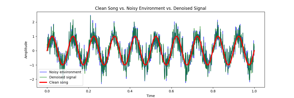
Generate and plot clean, noisy, and denoised signals to visualize the reconstruction

length = 1000
t, clean_signal = generate_clean_signal(length)
noisy_signal = add_noise(clean_signal, noise_level=0.5)
denoised_signal = fft_denoise(noisy_signal, threshold=10)

plt.figure(figsize=(12, 4))
plt.plot(t, noisy_signal, label="Noisy environment", color="blue", alpha=0.7)
plt.plot(t, denoised_signal, label="Denoised signal", color="green", alpha=0.7)
plt.plot(t, clean_signal, label="Clean song", color="red", linewidth=3)
plt.xlabel("Time")
plt.ylabel("Amplitude")
plt.title("Clean Song vs. Noisy Environment vs. Denoised Signal")
plt.legend()
plt.show()

Convert the signals to PyTorch tensors and calculate the SNR

clean_signal_tensor = torch.tensor(clean_signal).float()
noisy_signal_tensor = torch.tensor(noisy_signal).float()
denoised_signal_tensor = torch.tensor(denoised_signal).float()

snr = SignalNoiseRatio()
initial_snr = snr(preds=noisy_signal_tensor, target=clean_signal_tensor)
reconstructed_snr = snr(preds=denoised_signal_tensor, target=clean_signal_tensor)
print(f"Initial SNR: {initial_snr:.2f}")
print(f"Reconstructed SNR: {reconstructed_snr:.2f}")

Initial SNR: 3.19
Reconstructed SNR: 3.49

To show the effect of different noise levels on the SNR, we create an animation that iterates over different noise levels and updates the plot accordingly:

fig, ax = plt.subplots(figsize=(12, 4))
noise_levels = [0.1, 0.2, 0.3, 0.4, 0.5, 0.6, 0.7, 0.8, 0.9]


def update(num: int) -> tuple:
    """Update the plot for each frame."""
    t, clean_signal = generate_clean_signal(length)
    noisy_signal = add_noise(clean_signal, noise_level=noise_levels[num])
    denoised_signal = fft_denoise(noisy_signal, threshold=10)

    clean_signal_tensor = torch.tensor(clean_signal).float()
    noisy_signal_tensor = torch.tensor(noisy_signal).float()
    denoised_signal_tensor = torch.tensor(denoised_signal).float()
    initial_snr = snr(preds=noisy_signal_tensor, target=clean_signal_tensor)
    reconstructed_snr = snr(preds=denoised_signal_tensor, target=clean_signal_tensor)

    ax.clear()
    (noisy,) = plt.plot(t, noisy_signal, label="Noisy Environment", color="blue", alpha=0.7)
    (denoised,) = plt.plot(t, denoised_signal, label="Denoised Signal", color="green", alpha=0.7)
    (clean,) = plt.plot(t, clean_signal, label="Clean Song", color="red", linewidth=3)
    ax.set_xlabel("Time")
    ax.set_ylabel("Amplitude")
    ax.set_title(
        f"Initial SNR: {initial_snr:.2f} - Reconstructed SNR: {reconstructed_snr:.2f} - Noise level: {noise_levels[num]}"
    )
    ax.legend(loc="upper right")
    ax.set_ylim(-3, 3)
    return noisy, denoised, clean


ani = animation.FuncAnimation(fig, update, frames=len(noise_levels), interval=1000)

Once Loop Reflect