Key takeaway
Training and using large language models (LLMs) is expensive due to their large compute requirements and memory footprints. This article will explore how leveraging lower-precision formats can enhance training and inference speeds up to 3x without compromising model accuracy.
Although our primary focus will be on large language model examples, most of these techniques are versatile and applicable to other deep learning architectures as well.
Understanding Mixed-Precision Training
Mixed-precision training is one of the essential techniques that lets us significantly boost training speeds on modern GPUs. Sometimes, this can results in 2x to 3x speed-ups! Let’s see how this works.
Using 32-Bit Precision
When training deep neural networks on a GPU, we typically use a lower-than-maximum precision, namely, 32-bit floating point operations (in fact, PyTorch uses 32-bit floats by default).
In contrast, in conventional scientific computing, we typically use 64-bit floats. In general, a larger number of bits corresponds to a higher precision, which lowers the chance of errors accumulating during computations. As a result, 64-bit floating point numbers (also known as double-precision) have long been the standard in scientific computing due to their ability to represent a wide range of numbers with higher accuracy.
However, in deep learning, using 64-bit floating point operations is considered unnecessary and computationally expensive since 64-bit operations are generally more costly, and GPU hardware is also not optimized for 64-bit precision. So instead, 32-bit floating point operations (also known as single-precision) have become the standard for training deep neural networks on GPUs.
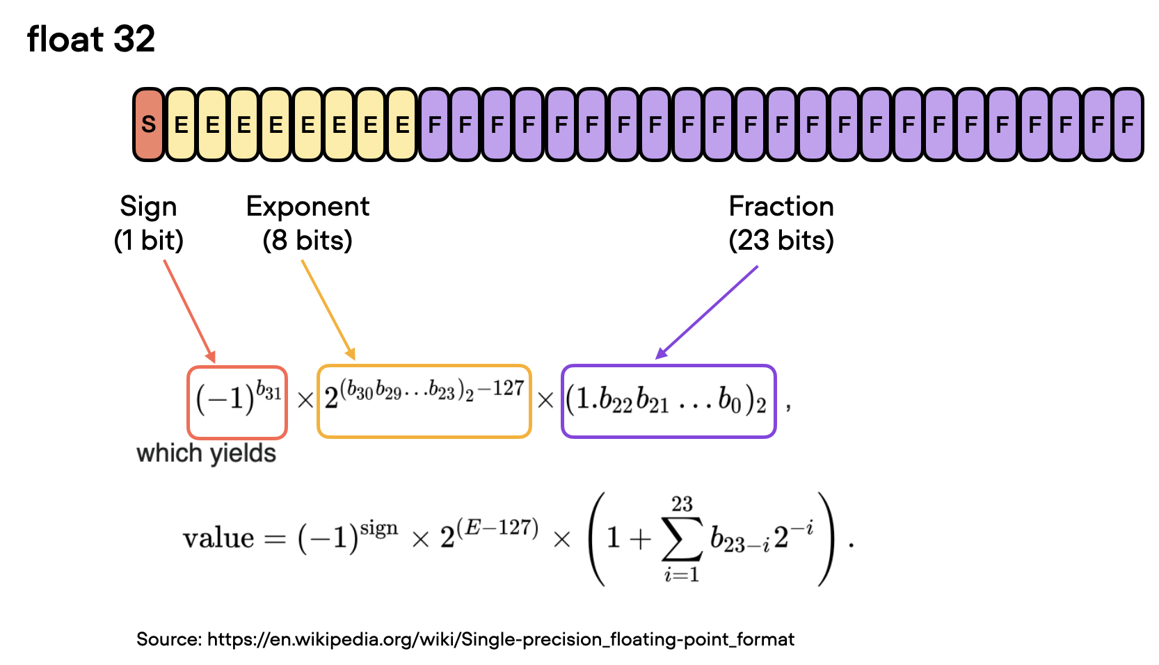
In the context of floating-point numbers, “bits” refer to the binary digits used to represent a number in a computer’s memory. The more bits used to represent a number, the higher the precision and the greater the range of values that can be represented. In floating-point representation, numbers are stored in a combination of three parts: the sign, the exponent, and the significand (or mantissa).
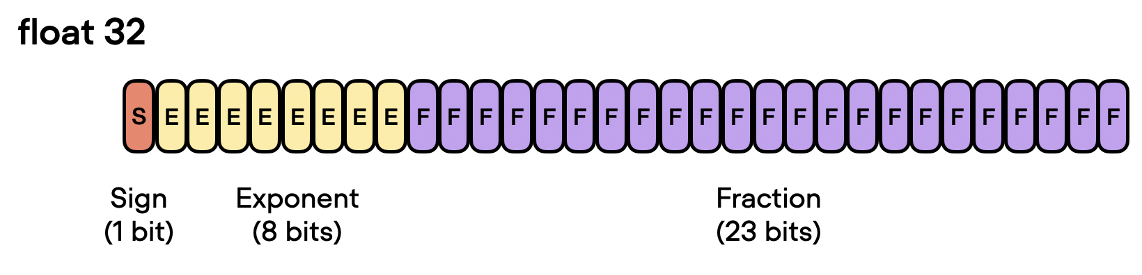
In a floating-point number, the value is represented as the product of the significand, the base raised to the exponent, and the sign. The significand is related but not equivalent to the digits after the decimal point. If you are interested in the exact formula (illustrated in the figure below), I recommend the excellent section on Wikipedia. However, for convenience, we can think of the significand as a “fraction” or “fractional value.”
So, coming back to the motivation behind using a lower precision, there are essentially two main reasons why 32-bit floating point operations are preferred over 64-bit when training deep neural networks on a GPU:
- Reduced memory footprint. One of the primary advantages of using 32-bit floats is that they require half the memory compared to 64-bit floats. This allows for more efficient use of GPU memory, enabling the training of larger models (and larger batch sizes).
- Increased compute and speed. Since 32-bit floating point operations require less memory, GPUs can process them more quickly, leading to faster training times. This speedup is crucial in deep learning, where training complex models can take days or even weeks.
From 32-Bit to 16-Bit Precision
Now that discussed the benefits of 32-bit floats, can we go even further? Yes, we can! Recently, mixed-precision training has become a common training scheme where we temporarily use 16-bit precision for floating point computation, which often referred to as “half” precision.
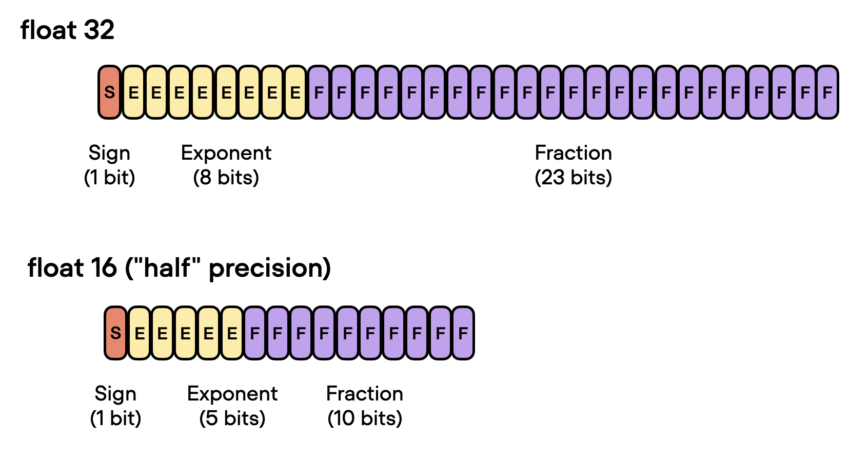
As shown in the figure above, float16 uses three fewer bits for the exponent and 13 fewer bits for the fractional value.
But before discussing the mechanics behind mixed-precision training, let’s make the difference between different bit-precision levels more intuitive and tangible. Consider the following code example in PyTorch:
>>> import torch
>>> torch.set_printoptions(precision=60)
>>> torch.tensor(1/3, dtype=torch.float64)
tensor(0.333333333333333314829616256247390992939472198486328125000000,
dtype=torch.float64)
>>> torch.tensor(1/3, dtype=torch.float32)
tensor(0.333333343267440795898437500000000000000000000000000000000000)
>>> torch.tensor(1/3, dtype=torch.float16)
tensor(0.333251953125000000000000000000000000000000000000000000000000,
dtype=torch.float16)
The code examples above show that the lower the precision, the fewer accurate digits we see after the decimal point.
Deep learning models are generally robust to lower precision arithmetic. In most cases, the slight decrease in precision from using 32-bit floats instead of 64-bit floats does not significantly impact the model’s predictive performance, making the trade-off worthwhile. However, things can become tricky when we go down to 16-bit precision. You may notice that the loss may become unstable or not converge due to imprecision, numeric overflow, or underflow.
Overflow and underflow refer to the issue that certain numbers exceed the range that can be handled by the precision format, for example, as demonstrated below:
>>> torch.tensor(10**6, dtype=torch.float32)
tensor(1000000.)
>>> torch.tensor(10**6, dtype=torch.float16)
tensor(inf, dtype=torch.float16)
By the way, while the code snippets above showed some hands-on examples regarding the different precision types, you can also directly access the numerical properties via torch.finfo as shown below:
>>>torch.finfo(torch.float32)
finfo(resolution=1e-06, min=-3.40282e+38, max=3.40282e+38,
eps=1.19209e-07, smallest_normal=1.17549e-38,
tiny=1.17549e-38, dtype=float32)
>>> torch.finfo(torch.float16)
finfo(resolution=0.001, min=-65504, max=65504,
eps=0.000976562, smallest_normal=6.10352e-05,
tiny=6.10352e-05, dtype=float16)
The code above reveals that the largest float32 number is 340,282,000,000,000,000,000,000,000,000,000,000,000 (via max); float16 numbers cannot exceed the value 65,504 for example.
So, in this section, we motivated using “mixed-precision” training rather than 16-bit precision training in modern deep learning. But how does this mixed-precision training work? And why is it called “mixed”-precision training instead of just 16-bit precision training? Let’s answer these questions in the section below.
Mixed-Precision Training Mechanics
It’s called “mixed-” rather than “low-“precision training because we don’t transfer all parameters and operations to 16-bit floats. Instead, we switch between 32-bit and 16-bit operations during training, hence, the term “mixed” precision.
As illustrated in the figure below, mixed-precision training involves converting weights to lower-precision (FP16) for faster computation, calculating gradients, converting gradients back to higher-precision (FP32) for numerical stability, and updating the original weights with the scaled gradients.
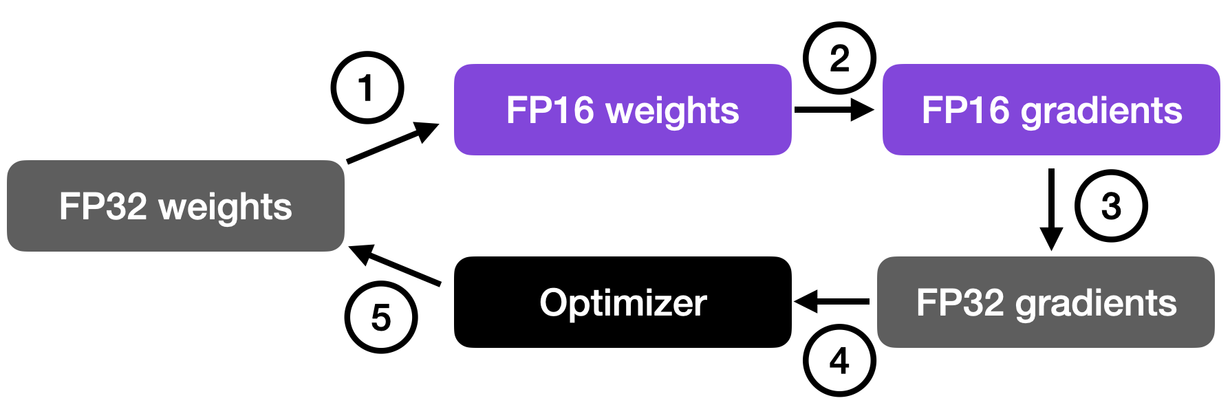
This approach allows for efficient training while maintaining the accuracy and stability of the neural network.
In more detail, the steps are as follows.
- Convert weights to FP16: In this step, the weights (or parameters) of the neural network, which are initially in FP32 format, are converted to lower-precision FP16 format. This reduces the memory footprint and allows for faster computation, as FP16 operations require less memory and can be processed more quickly by the hardware.
- Compute gradients: The forward and backward passes of the neural network are performed using the lower-precision FP16 weights. This step calculates the gradients (partial derivatives) of the loss function with respect to the network’s weights, which are used to update the weights during the optimization process.
- Convert gradients to FP32: After computing the gradients in FP16, they are converted back to the higher-precision FP32 format. This conversion is essential for maintaining numerical stability and avoiding issues such as vanishing or exploding gradients that can occur when using lower-precision arithmetic.
- Multiply by learning rate and update weights: Now in FP32 format, the gradients are multiplied by a learning rate (a scalar value that determines the step size during optimization).
- The product from step 4 is then used to update the original FP32 neural network weights. The learning rate helps control the convergence of the optimization process and is crucial for achieving good performance.
The above procedure sounds quite complicated, but in practice, it’s pretty simple to implement. In the next section, we will see how we can use mixed-precision training for finetuning an LLM by changing just one line of code.
A Mixed-Precision Code Example
Using PyTorch’s autocast context manager, mixed-precision training is fortunately not very complicated. Furthermore, with the open-source Fabric library for PyTorch, flipping between regular and mixed-precision training is even more accessible and only requires changing one line of code. (Due to lack of manual intervention or modification of the training code, this is often also called automatic mixed-precision training.)
So, first, we will look at an encoder-LLM that we finetune for a supervised classification task (here: DistilBERT for classifying the sentiment of movie reviews) in terms of runtime, prediction accuracy, and memory requirements. In particular, we are going to finetune all layers of the transformer. For more information about the different types of finetuning, see my previous Understanding Parameter-Efficient Finetuning of Large Language Models article and Unit 8.7, A Large Language Model for Classification, or my free Deep Learning Fundamentals course.
Later, we will also see how the choice of the different precision levels impacts large language models like LLaMA.
Finetuning Benchmarks
Let’s start with the code for finetuning a DistilBERT model in regular fashion with float32 bit precision, which is the default in PyTorch:
from datasets import load_dataset
from lightning import Fabric
import torch
from torch.utils.data import DataLoader
import torchmetrics
from transformers import AutoTokenizer
from transformers import AutoModelForSequenceClassification
##########################
### 1 Loading the Dataset
##########################
# ... omitted for brevity
#########################################
### 2 Tokenization and Numericalization
#########################################
# ... omitted for brevity
#########################################
### 3 Set Up DataLoaders
#########################################
# ... omitted for brevity
#########################################
### 4 Initializing the Model
#########################################
fabric = Fabric(accelerator="cuda", devices=1)
fabric.launch()
model = AutoModelForSequenceClassification.from_pretrained(
"distilbert-base-uncased", num_labels=2)
optimizer = torch.optim.Adam(model.parameters(), lr=5e-5)
model, optimizer = fabric.setup(model, optimizer)
train_loader, val_loader, test_loader = fabric.setup_dataloaders(
train_loader, val_loader, test_loader)
#########################################
### 5 Finetuning
#########################################
start = time.time()
train(
num_epochs=3,
model=model,
optimizer=optimizer,
train_loader=train_loader,
val_loader=val_loader,
fabric=fabric
)
#########################################
### 6 Evaluation
#########################################
# ... omitted for brevity
print(f"Time elapsed {elapsed/60:.2f} min")
print(f"Memory used: {torch.cuda.max_memory_reserved() / 1e9:.02f} GB")
print(f"Test accuracy {test_acc.compute()*100:.2f}%")
The code above is abbreviated to save space, but you can access the full code examples here on GitHub.
The results from training on a single A100 GPU are as follows:
Python implementation: CPython
Python version : 3.9.16
torch : 2.0.0
lightning : 2.0.2
transformers: 4.28.1
Torch CUDA available? True
...
Train acc.: 97.28% | Val acc.: 89.88%
Time elapsed 21.75 min
Memory used: 5.37 GB
Test accuracy 89.92%
Now, to compare it to float16 mixed-precision training, we only have to change one line of code, from
fabric = Fabric(accelerator="cuda", devices=1)
to
fabric = Fabric(accelerator="cuda", devices=1, precision="16-mixed")
The results are as follows:
Train acc.: 97.39% | Val acc.: 92.21%
Time elapsed 7.25 min
Memory used: 4.31 GB
Test accuracy 92.15%
Above, we can see that the required memory reduced, likely as a consequence of carrying out the matrix multiplications in 16-bit precision. Furthermore, the training speed improved approximately 3-fold, which is huge.
An interesting, unexpected observation is that the prediction accuracy improved as well. A likely explanation is that this is due to regularizing effects of using a lower precision. Lower precision may introduce some level of noise in the training process, which can help the model generalize better and reduce overfitting, potentially leading to higher accuracy on the validation and test sets.
Out of curiosity, we will also add the results for regular (not mixed) float16 training via
fabric = Fabric(accelerator="cuda", devices=1, precision="16-full")
(Note that this currently requires installing Lightning from the latest developer branch via
pip install git+https://github.com/Lightning-AI/lightning@master.)Unfortunately, this results in non-convergence of the loss, hence, the accuracy is equal to a random prediction on this dataset (50%).
epoch: 0003/0003 | Batch 2700/2916 | Loss: nan
Epoch: 0003/0003 | Train acc.: 49.86% | Val acc.: 50.80%
Time elapsed 5.23 min
Memory used: 2.87 GB
Test accuracy 50.08%
The results from above are summarized in the following chart:
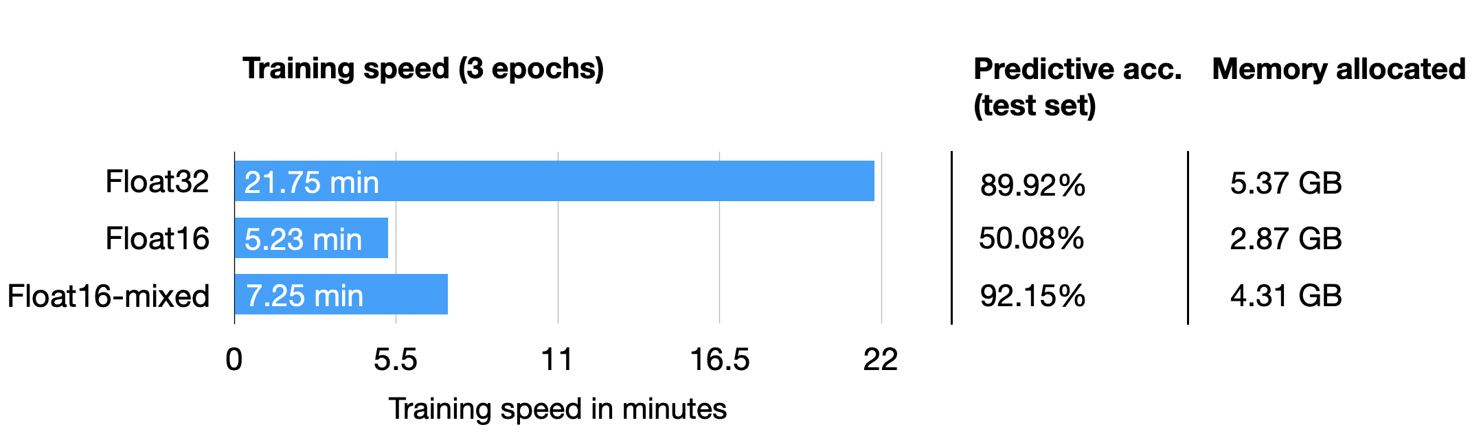
As we can see, float16 mixed-precision is almost as fast as pure float16 precision training (which has numeric problems here) and outperforms float32 predictive performance as well, likely due to the regularizing effect discussed above.
Tensor Cores and Matrix Multiplication Precision
By the way, if you are running the previous code on a GPU that supports tensor cores, you may have seen the following message via PyTorch in the terminal:
You are using a CUDA device ('NVIDIA A100-SXM4-40GB') that has Tensor Cores.
To properly utilize them, you should
set `torch.set_float32_matmul_precision('medium' | 'high')`
which will trade-off precision for performance.
For more details,
read https://pytorch.org/docs/stable/generated/torch.
set_float32_matmul_precision.html#torch.set_float32_matmul_precision
So, by default, PyTorch uses the “highest” precision for matrix multiplications. But if we want to trade off more precision for performance (as described in the PyTorch docs here), you can also set
torch.set_float32_matmul_precision("high")
or
torch.set_float32_matmul_precision("medium")
(The default is usually “highest”.)
The settings above will utilize a bfloat16 datatype for matrix multiplications, which is a special type of float16 — more details on the bfloat16 type in the next section. So, in other words, using torch.set_float32_matmul_precision("high"/"medium") will implicitly enable a flavor of mixed precision training (via matrix multiplications) if your GPU supports tensor cores.
How does this affect the results? Let’s have a look:
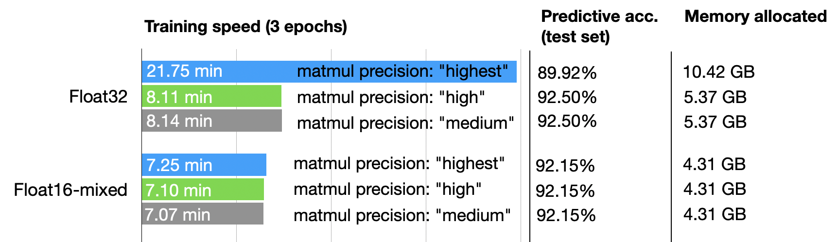
So, as we can see above, for float32 precision, lowering the matrix multiplication precision has a significant effect, improving the computational performance 2.5x and halving the memory requirements. Also, the predictive accuracy increases, likely due to the regularizing effects of lower precision mentioned earlier.
In fact, using float32 training with lower matrix multiplication precision almost equals float16 mixed-precision training in terms of performance. Furthermore, enabling lower matrix multiplication precision for float16 does not improve the results because float16 mixed-precision training already uses float16 precision for matrix multiplications.
Brain Floating Point
Another floating-point format has recently gained popularity, Brain Floating Point (bfloat16). Google developed this format for machine learning and deep learning applications, particularly in their Tensor Processing Units (TPUs). Bfloat16 extends the dynamic range compared to the conventional float16 format at the expense of decreased precision.
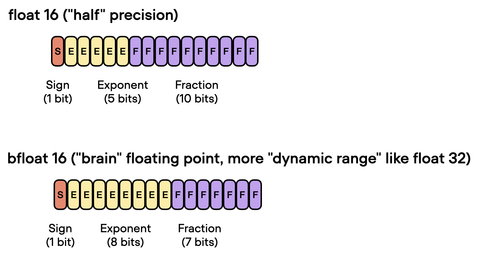
The extended dynamic range helps bfloat16 to represent very large and very small numbers, making it more suitable for deep learning applications where a wide range of values might be encountered. However, the lower precision may affect the accuracy of certain calculations or lead to rounding errors in some cases. But in most deep learning applications, this reduced precision has minimal impact on modeling performance.
While bfloat16 was originally developed for TPUs, this format is now supported by several NVIDIA GPUs as well, beginning with the A100 Tensor Core GPUs, which are part of the NVIDIA Ampere architecture.
You can check whether your GPU supports bfloat16 via the following code:
>>> torch.cuda.is_bf16_supported()
True
Can bfloat16 benefit us further? To answer this question, let’s add the bfloat16 results from running the previous DistilBERT code by changing one line of code from
fabric = Fabric(accelerator="cuda", devices=1, precision="16-mixed")
to
fabric = Fabric(accelerator="cuda", devices=1, precision="bf16-mixed")
(The full scripts are available on GitHub here.)
For completeness, I am also adding the results for a float64 run. And for fun, let’s also try out regular (not mixed-precision) bfloat16 training:
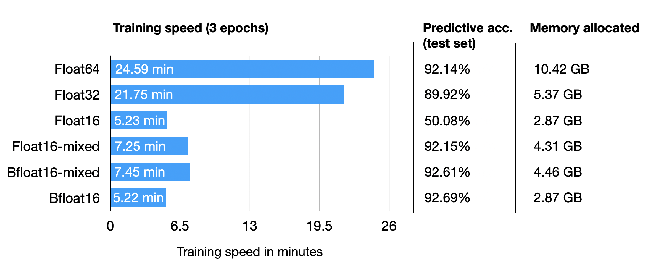
Interestingly, float64 achieves a higher accuracy than float32 here, which contradicts our previous argument of lower precision having a regularizing effect on this model. However, the interesting point is that Bfloat16 mixed-precision training (92.61%) improves the results slightly compared to Float16 (92.15%) mixed-precision training regarding predictive performance; it uses a bit more memory, though. Note that we cannot include regular Float16 (50%) training in the comparison, since it doesn’t train properly due to the low-precision.
All in all, float16 and bfloat16 mixed-precision training behave relatively similarly here, which is not unexpected.
And interestingly, the larger dynamic range of bfloat16 also allows us to train the model without mixed-precision training, where regular float16 training fails. Note that this is a lucky coincidence here, and in many cases, I experienced that full bfloat16 training does not work as well as bfloat16 mixed-precision training.
Efficient Lower-Precision Inference and LLaMA
Mixed-precision training can be extended to inference in deep learning models to improve efficiency, reduce memory footprint, and accelerate computation. However, we must keep in mind that applying lower precision during inference may result in a slight degradation of model accuracy due to the reduced numerical precision. However, in many deep learning applications, the impact on accuracy is minimal and is an acceptable trade-off for the benefits of reduced memory usage and faster computation.
In fact, the mixed-precision finetuning codes above already used a 16-bit precision for inference via the Fabric setting when computing the training, validation, and test set accuracies. Since DistilBERT is a relatively small model, the inference speed is only a tiny fraction of the total runtime.
So, to include a slightly more interesting inference example, let’s look at Meta’s popular LLaMA model for generating text. Here, we will use the user-friendly Lit-LLaMA repository, which uses the same Fabric code to implement the 16-precision we used earlier.
However, since pretraining a large language model on terabytes of data is relatively expensive, we will use Meta’s existing model checkpoints to evaluate the model during inference, generating new text.

If you use the repository for the first time, see the Setup section to install the requirements and how-to guide for downloading the weights.
After the repository is set up, we can use the generate.py script to generate text following a prompt, which uses bfloat16 by default:
python generate.py --prompt "Large language models are" # uses bfloat16
Loading model ...
Time to load model: 24.84 seconds.
Global seed set to 1234
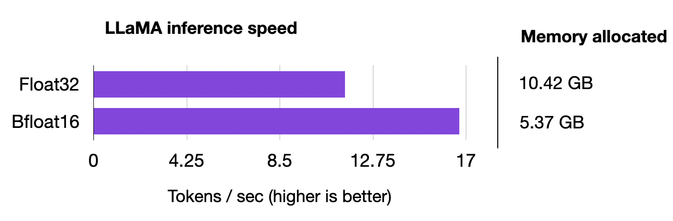
Large language models are an effective solution to the sequential inference task of natural language understanding, but are unfeasible for mobile applications. In this paper, we investigate a simple, yet effective approach to reduce the computational and memory demands of large language models by removing
Time for inference 1: 2.99 sec total, 16.70 tokens/sec
Memory used: 13.52 GB
To compare it to float32 precision, we have to modify the script manually, changing the Fabric device type from torch.bfloat16 to torch.float32.
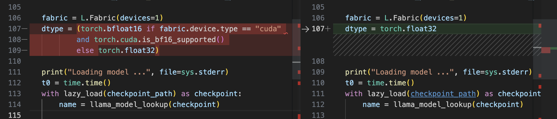
After this modification, let’s rerun the generate.py scripts with the same prompt as above:
python generate.py \
--prompt "Large language models are" # disabled bfloat16, using float32
Loading model ...
Time to load model: 17.93 seconds.
Global seed set to 1234
Large language models are an effective solution to the sequential
data modelling tasks, but the huge size of these models makes them
difficult to learn due to the large amount of parameters and the
time to train them. The high computational cost, as well as the
long training times
Time for inference 1: 4.36 sec total, 11.47 tokens/sec
Memory used: 27.02 GB
We can see that the model uses twice as much memory now, and the model is now 30% slower.
Quantization
If we want to increase the model performance during inference even more, we can also move beyond lower floating point precision and use quantization. Quantization converts the model weights from floats to low-bit integer representations, for example, 8-bit integers (and, recently, even 4-bit integers).
However, since this is already a long blog post, we will defer a more detailed explanation to a future article.
In the meantime, both int8 quantization (LLM.int8(): 8-bit Matrix Multiplication for Transformers at Scale) and int4 quantization (GPTQ: Accurate Post-Training Quantization for Generative Pre-trained Transformers) are already supported in Lit-LLaMA if you want to give it a try!
Conclusion
In this article, we saw how we could significantly boost the training speed of an LLM classifier 3-fold using 16-bit precision techniques. In addition, we are also able to cut the memory consumption in half!
Moreover, we looked at the inferencing speeds of generative AI models and were able to boost the performance by 30% as well while doubling memory efficiency.
So, if you use a GPU that supports mixed-precision training, it’s worth utilizing it since it’s as simple as changing a single line of code!
Acknowledgements
I want to thank Luca Antiga and Adrian Waelchli for the constructive feedback to improve the clarity of this article.