Takeaways
This guide targets PyTorch model training, illustrating how you can adjust the floating point precision to drastically enhance training speed and halve memory consumption, all without compromising the prediction accuracy.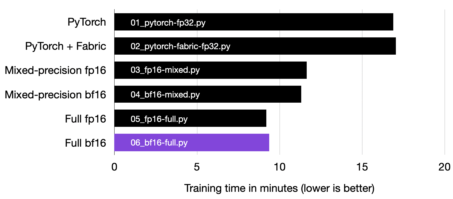
An excerpt of the improvements we can gain from leveraging the techniques introduced in this article.
In this article, we will work with a vision transformer from PyTorch’s Torchvision library, providing simple code examples that you can execute on your own machine without the need to download and install numerous code and dataset dependencies. The self-contained baseline training script comprises approximately 100 lines of code, excluding whitespace and code comments.
All benchmarks were executed using the open source Lightning 2.1 package with PyTorch 2.1 and CUDA 12.1 on a single A100 GPU. You can find all code examples here on GitHub.
Finetuning a Vision Transformer on a Single GPU
While we are working with a vision transformer here (the ViT-L-16 model from the paper
An Image is Worth 16×16 Words: Transformers for Image Recognition at Scale), all the techniques used in this article transfer to other models as well: Convolutional networks, large language models (LLMs), and others.
Note that we are finetuning the model for classification instead of training it from scratch to optimize predictive performance.
Let’s begin with a simple baseline in PyTorch. The complete code is available here on GitHub, which implements and finetunes a vision transformer:
The core code for implementing this vision transformers is as follows:
# Import torchvision
from torchvision.models import vit_l_16
from torchvision.models import ViT_L_16_Weights

# Initialize pretrained vision transformer
model = vit_l_16(weights=ViT_L_16_Weights.IMAGENET1K_V1)

# replace output layer
model.heads.head = torch.nn.Linear(in_features=1024, out_features=10)

# finetune model
The relevant benchmark numbers for this baseline are as follows:
- Training runtime: 16.88 min
- GPU memory: 16.70 GB
- Test accuracy: 94.06%
Introducing the Open Source Fabric Library
To simplify the PyTorch code for the experiments, we will be introducing the open-source Fabric library, which allows us to apply various advanced PyTorch techniques (automatic mixed-precision training, multi-GPU training, tensor sharding, etc.) with a handful (instead of dozens) lines of code.
The difference between simple PyTorch code and the modified one to use Fabric is subtle and involves only minor modifications, as highlighted in the code below.
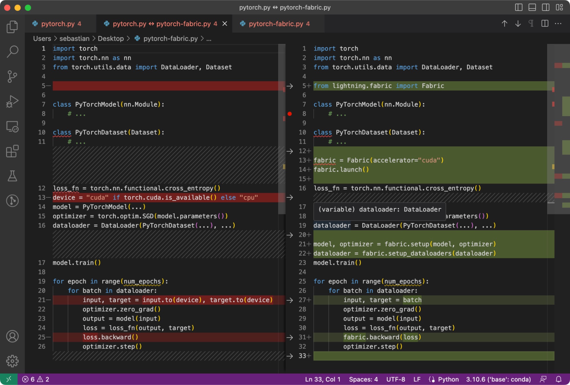
It requires only a handful of changes to utilize the open-source Fabric library for PyTorch model training.
As mentioned above, these minor changes now provide a gateway to utilize advanced features in PyTorch, as we will see in a bit, without restructuring any more of the existing code.
To summarize the figure above, the main 3 steps for converting plain PyTorch code to PyTorch+Fabric are as follows:
Since Fabric is a wrapper around PyTorch, it should not affect the runtime of our code, a fact we can confirm via the performance benchmarks below.
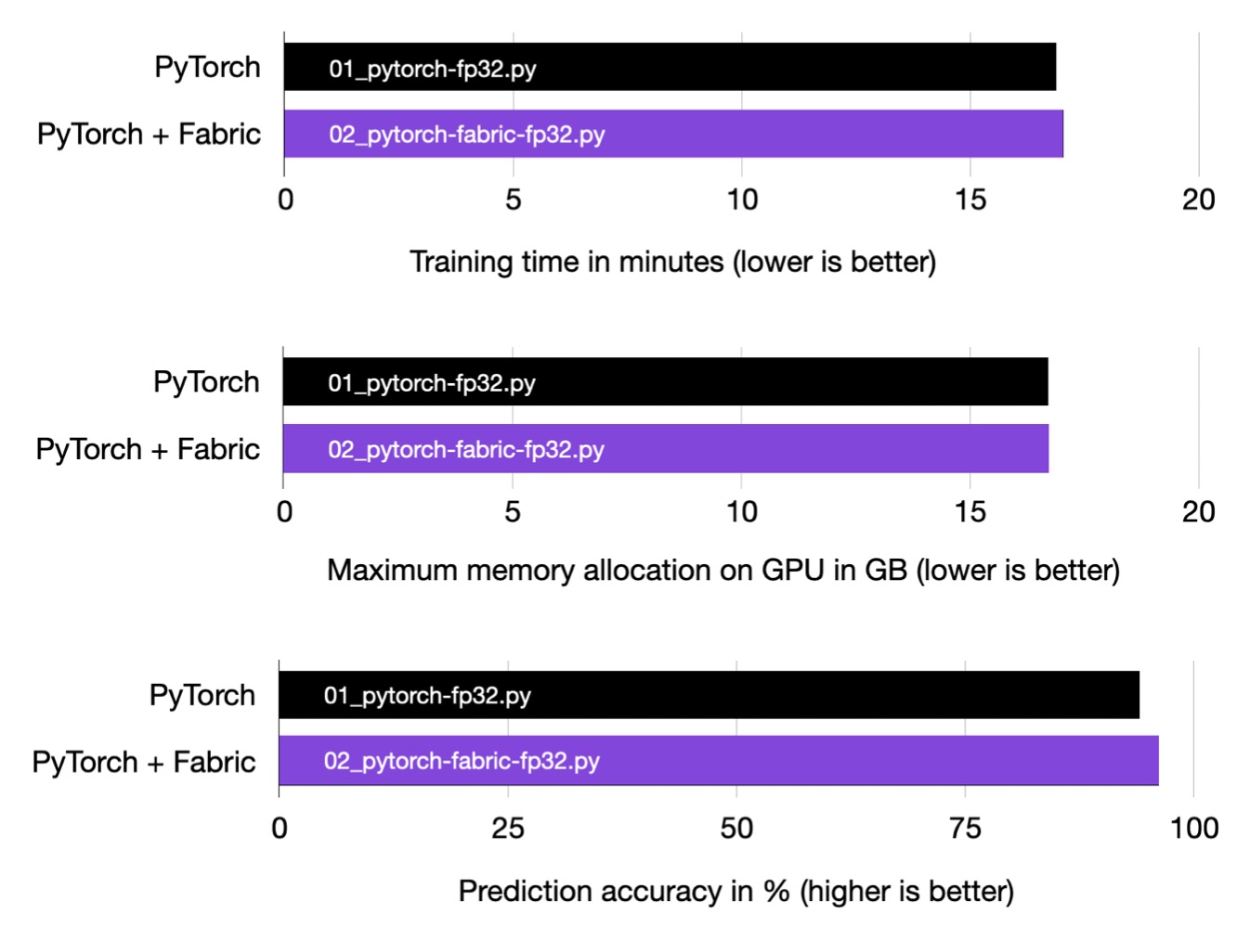
Training time, memory usage, and prediction accuracy are the same for plain PyTorch and PyTorch augmented with Fabric.
Note that if there are minor differences in the bar plots above, these can be attributed to the randomness inherent in training neural networks and machine fluctuations. If we were to repeat the runs multiple times and examine the averaged results, the bar plots would be exactly the same.
16-bit Mixed Precision Training
In the previous section, we modified our PyTorch code using Fabric. Why go through all this hassle? As we will see below, we can now try advanced techniques, like mixed-precision training, by only changing one line of code. (Similarly, we can enable distributed training in one line of code, but this is a topic for a different article.)
Using Mixed-Precision Training
We can use mixed-precision training with only one small modification, changing
fabric = Fabric(accelerator="cuda", devices=1)
to the following:
fabric = Fabric(accelerator="cuda", devices=1, precision="16-mixed")
As we can see in the charts below, using mixed-precision training, we cut down the training time by more than 30%. We also improved the peak memory consumption by more than 25% while maintaining the same prediction accuracy. Based on my personal experience, I observed even more significant gains when working with larger models.
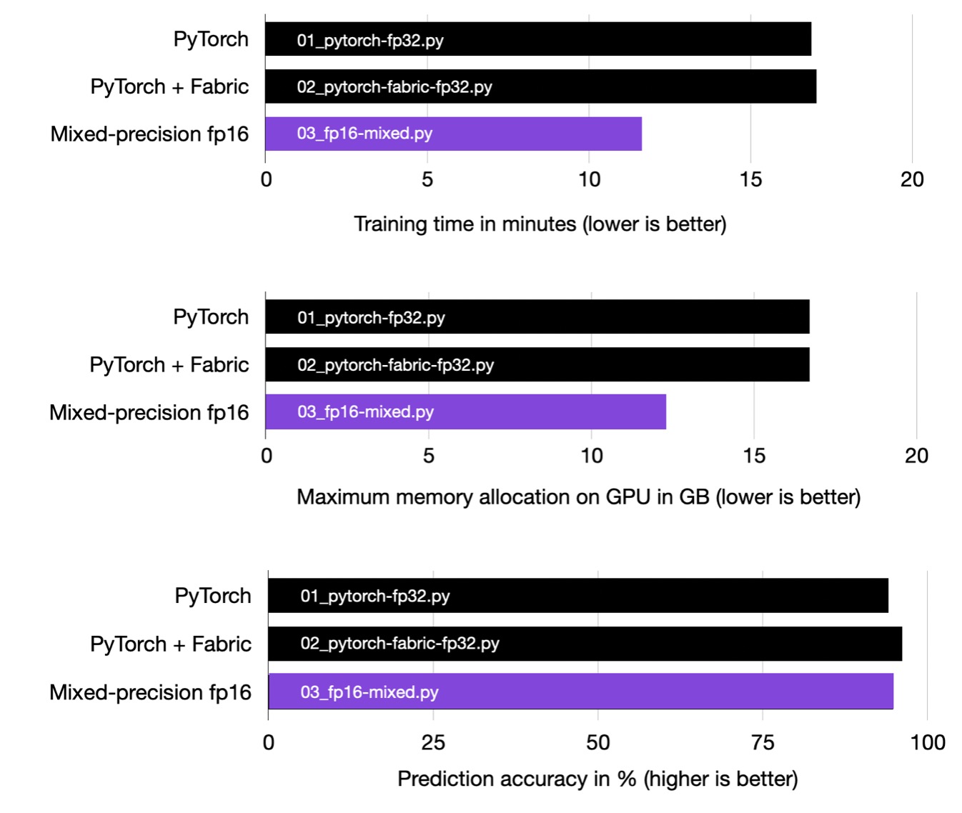
Mixed-precision training significantly reduces training time and memory consumption.
What Is Mixed-Precision Training?
Mixed precision training utilizes both 16-bit and 32-bit precision to ensure no loss in accuracy. The computation of gradients in 16-bit representation is much faster than in 32-bit format, which also saves a significant amount of memory. This strategy is particularly beneficial when we are constrained by memory or computational resources.
The term “mixed” rather than “low” precision training is used because not all parameters and operations are transferred to 16-bit floats. Instead, we alternate between 32-bit and 16-bit operations during training, hence the term “mixed” precision.
As illustrated in the figure below, mixed precision training involves converting weights to lower precision (16-bit floats, or FP16) for faster computation, calculating gradients, converting gradients back to higher precision (FP32) for numerical stability, and updating the original weights with the scaled gradients.
This approach enables efficient training while maintaining the accuracy and stability of the neural network.
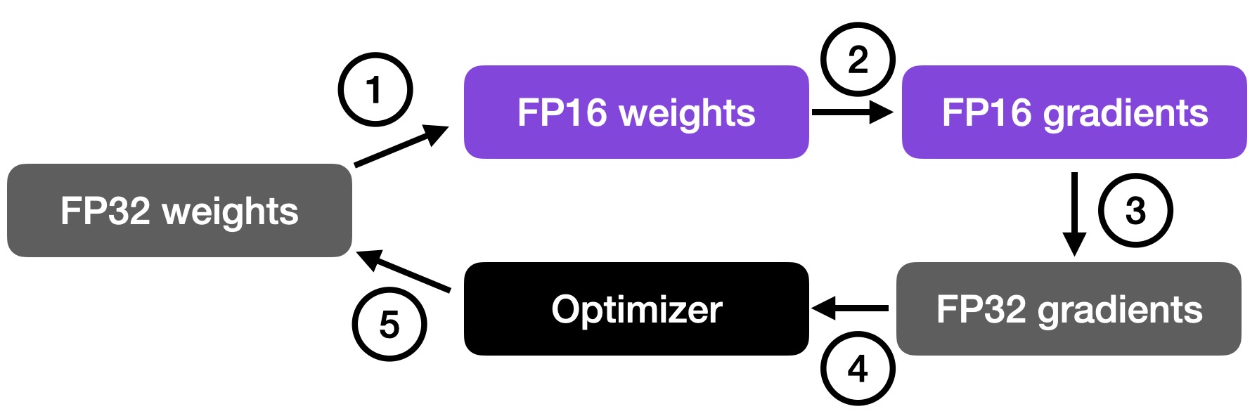
An overview of mixed-precision training. For additional details, I also cover this concept in Unit 9.1 of my Deep Learning Fundamentals class.
Full 16-bit Precision Training
We can also take it a step further and attempt running with “full” lower 16-bit precision, as opposed to mixed precision, which converts intermediate results back to a 32-bit representation.
We can enable lower-precision training by changing
fabric = Fabric(accelerator="cuda", precision="16-mixed")
to the following:
fabric = Fabric(accelerator="cuda", precision="16-true")
(Note that “16-true” is a new feature in Lightning 2.1 and is not available in older versions.)
However, you may notice that when running this code, you’ll encounter NaN values in the loss:
Epoch: 0001/0001 | Batch 0000/0703 | Loss: 2.4105
Epoch: 0001/0001 | Batch 0300/0703 | Loss: nan
Epoch: 0001/0001 | Batch 0600/0703 | Loss: nan
...
This is because regular 16-bit floats can only represent numbers between -65,504 and 65,504:
In [1]: import torch
In [2]: torch.finfo(torch.float16)
Out[2]: finfo(resolution=0.001, min=-65504, max=65504, eps=0.000976562, smallest_normal=6.10352e-05, tiny=6.10352e-05, dtype=float16)
To avoid this NaN issue, we can use bfloat16, an alternative to 16-bit floating points, which will be discussed in the next section.
Full 16-bit Precision Training with BFloat-16
To circumvent the NaN issue we encountered with full 16-bit precision training in the previous section, we can utilize an alternative 16-bit format called bfloat16. This can be implemented using the “bf16-true” setting in Fabric:
fabric = Fabric(accelerator="cuda", precision="bf16-true")
(Note that bfloat16 can also be used for mixed precision training, and the results are included in the chart below.)
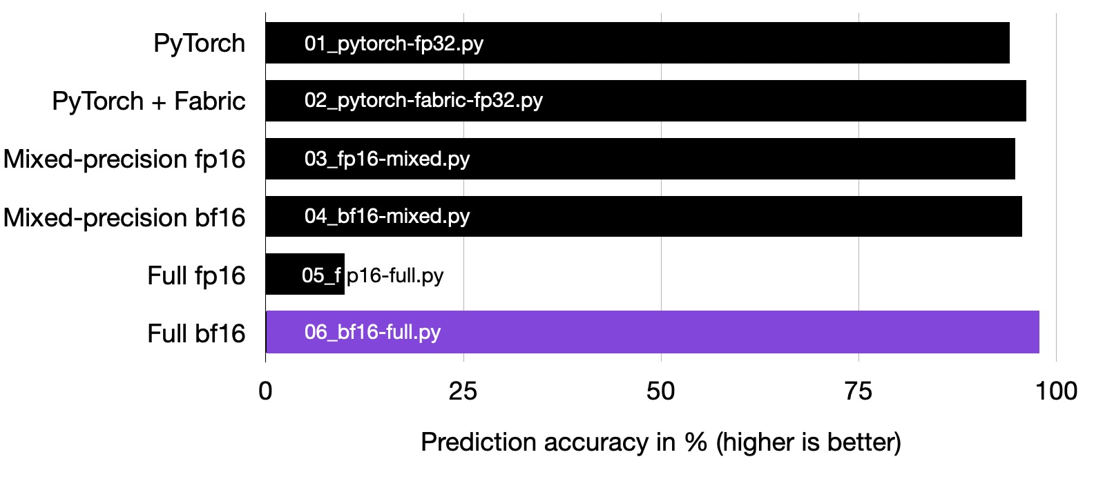
Full bfloat16 training does not suffer from the same stability issues as regular 16-bit precision training for this particular vision transformer.
But more impressively, by employing full bfloat16 training, we can achieve another significant improvement over mixed-precision training in terms of speed. And compared to the original 32-bit floating point training, which is the default option in deep learning (the first row, 01_pytorch-fp32.py), we can halve the training time.
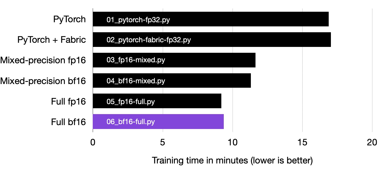
Full bfloat16 training is substantially faster than mixed-precision training, and it is about twice as fast as regular 32-bit precision training.
Just as using the bfloat16 format can halve training time, it also offers substantial memory savings, allowing us to train larger models on smaller GPUs.
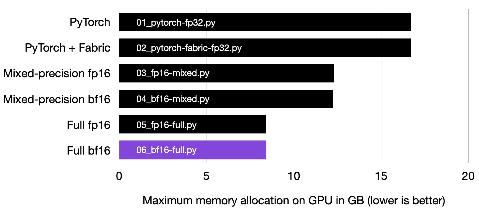
Bf16-training requires substantially less memory compared to mixed-precision training.
In my experiments, full bfloat16 training didn’t compromise prediction accuracy. However, this might not hold true for all models. When working with new architectures, it’s crucial to verify this. If you observe a decline in predictive performance with bfloat16 (even after running the training for just a few epochs or iterations), I recommend transitioning to 16-mixed or b16-mixed. Mixed precision training typically matches the performance of full 32-bit training.
What Is Bfloat16?
The “bf16” in “bf16-true” stands for Brain Floating Point (bfloat16). Google developed this format for machine learning and deep learning applications, particularly in their Tensor Processing Units (TPUs). Bfloat16 extends the dynamic range compared to the conventional float16 format at the expense of decreased precision.
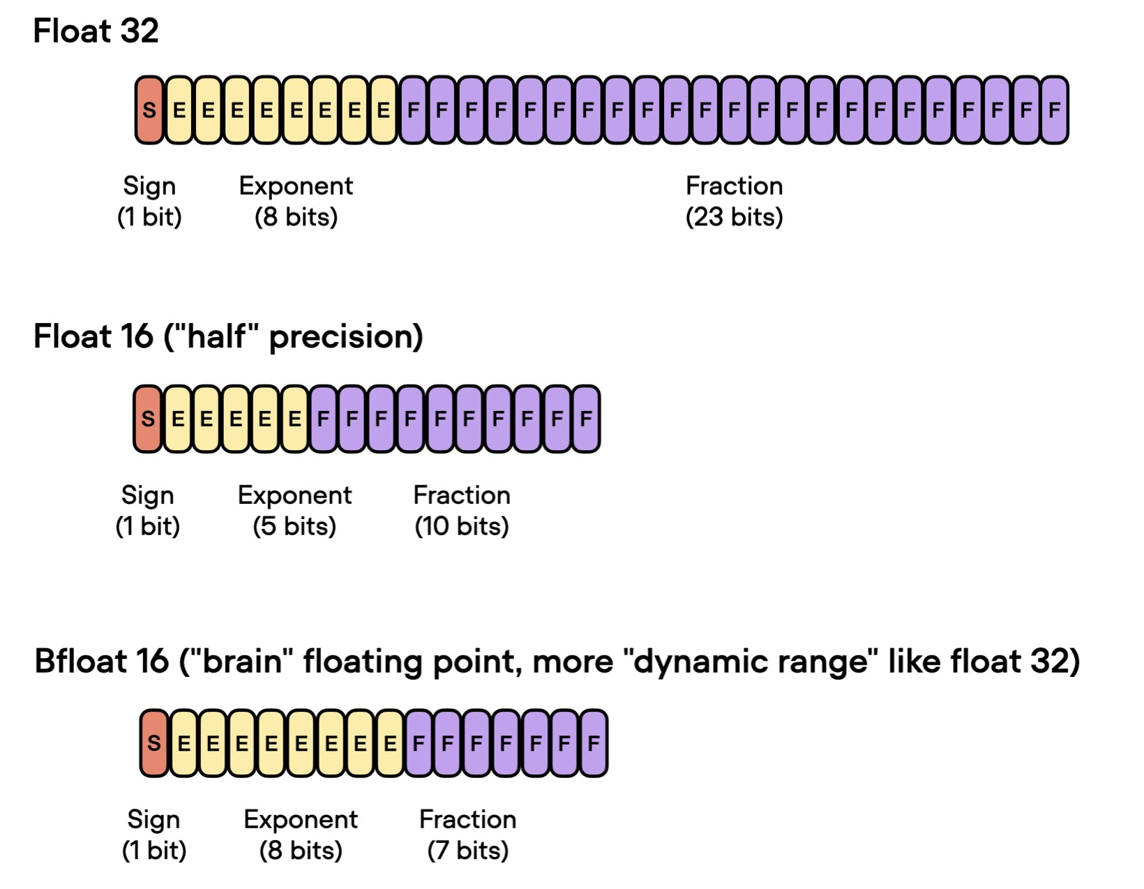
Bfloat16’s extended dynamic range allows it to represent very large and very small numbers effectively, making it well-suited for deep learning applications with their wide value ranges.
Although its lower precision could impact certain calculations or introduce rounding errors, this typically has a negligible effect on the overall performance in many deep learning tasks.
Initially developed for TPUs, bfloat16 is now also supported by various NVIDIA GPUs, starting with the A100 Tensor Core GPUs that belong to the NVIDIA Ampere architecture.
You can check whether your GPU supports bfloat16 via the following code:
>>> import torch
>>> torch.cuda.is_bf16_supported()
True
Conclusion
In this article, we explored how low-precision training techniques can speed up PyTorch model training by a factor of 2 and halve peak memory consumption. This enables the training of larger models on less expensive hardware. Notably, employing full bfloat16 precision, which is now supported in Lightning 2.1, was able to preserve the model’s prediction accuracy, so using it can be a cost-effective and efficient strategy for scaling deep learning tasks without sacrificing performance.
If you found this article useful, consider sharing it with your colleagues. For any questions or suggestions, feel free to join our Discord community.