Finetuning LLMs with LoRA and QLoRA: Insights from Hundreds of Experiments

Introduction: Getting the Most out of LoRA

I’ve run hundreds, if not thousands, of experiments involving LoRA over the past few months. A few weeks ago, I took the time to delve deeper into some of the hyperparameter choices.

This is more of an experimental diary presented in sequential order. I hope it proves useful to some. Specifically, I aim to address questions about the value of QLoRA, whether to replace AdamW with SGD, the potential use of a scheduler, and how to adjust the LoRA hyperparameters.

There’s a lot to discuss on the experimental side, so I’ll keep the introduction to LoRA brief.

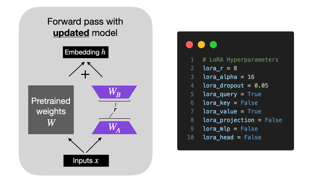
In short, LoRA, short for Low-Rank Adaptation (Hu et al 2021), adds a small number of trainable parameters to the model while the original model parameters remain frozen.

LoRA decomposes a weight matrix into two smaller weight matrices, as illustrated below, to approximate full supervised finetuning in a more parameter-efficient manner.

For more details about LoRA, please see my in-depth article Parameter-Efficient LLM Finetuning With Low-Rank Adaptation (LoRA).

The topics we are going to cover in this article as organized as follows:

1. Evaluation Tasks and Dataset
2. Code Framework
3. Choosing a Good Base Model
4. Evaluating the LoRA Defaults
5. Memory Savings with QLoRA
6. Learning Rate Schedulers and SGD
7. Iterating Over the Dataset Multiple Times
8. LoRA Hyperparameter Tuning Part 1: LoRA for All Layers
9. LoRA Hyperparameter Tuning Part 2: Increasing R
10. LoRA Hyperparameter Tuning Part 3: Changing Alpha
11. LoRA Hyperparameter Tuning Part 3: Very Large R
12. Leaderboard Submission
13. Conclusion

Evaluation Tasks and Dataset

The focus of this article is on selecting the optimal settings. To stay within a reasonable scope, I’m keeping the dataset fixed and focusing solely on supervised instruction-finetuning of LLMs. (Modifications to the dataset or finetuning for classification might be addressed in future articles.)

For the model evaluation, I selected a small subset of tasks from Eleuther AI’s Evaluation Harness, including TruthfulQA, BLiMP Causative, MMLU Global Facts, and simple arithmetic tasks with two (arithmetic 2ds) and four digits (arithmetic 4ds).

In each benchmark, the model performance score is normalized between 0 and 1, where 1 is a perfect score. TruthfulQA reports two scores, which are defined as follows:

• MC1 (Single-true): Given a question and 4-5 answer choices, select the only correct answer. The model’s selection is the answer choice to which it assigns the highest log-probability of completion following the question, independent of the other answer choices. The score is the simple accuracy across all questions.
• MC2 (Multi-true): Given a question and multiple true / false reference answers, the score is the normalized total probability assigned to the set of true answers.

For reference, the 175B GPT-3 model has TruthfulQA MC1 and MC2 values of 0.21 and 0.33, respectively.

Below are two examples to illustrate the difference between arithmetic 2ds and arithmetic 4ds:

• Arithmetic 2ds: “What is 59 minus 38”. “21”.
• Arithmetic 4ds: “What is 2762 plus 2751”. “5513”.

As mentioned above, I kept the dataset fixed, using the well-studied or rather commonly used Alpaca dataset for supervised instruction finetuning. Of course, many other datasets are available for instruction finetuning, including LIMA, Dolly, LongForm, FLAN, and more. However, exploring training on multiple datasets and dataset mixes will be an interesting topic for future studies.

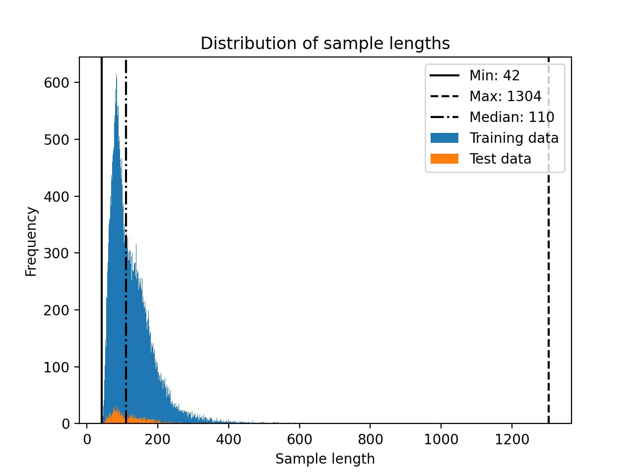
The Alpaca dataset consists of approximately 50k instruction-response pairs for training with a median length of 110 tokens for the input size (using the Llama 2 SentencePiece tokenizer), as shown in the histogram below.

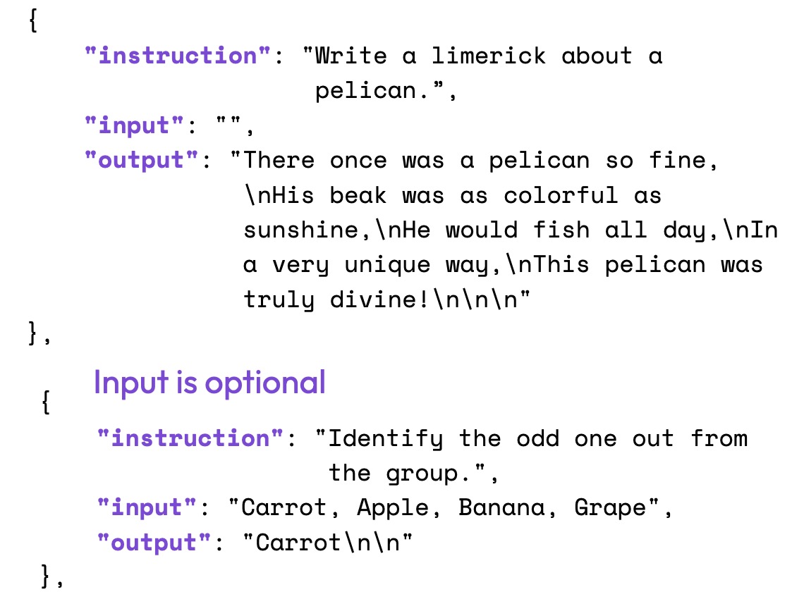
The dataset tasks themselves can be structured as shown in the figure below.

Code Framework

The custom LLM finetuning code I used for this article is based on the open-source Lit-GPT repository. To keep the preamble of this article brief, I won’t go into the usage details, but you can find a more detailed guide in the Lit-GPT tutorials section here.

In brief, the usage is as follows:

1) Clone the repository and install the requirements

git clone https://github.com/Lightning-AI/lit-gpt

cd lit-gpt

pip install -r requirements.txt

2) Download and prepare a model checkpoint

python scripts/download.py \
  --repo_id mistralai/Mistral-7B-Instruct-v0.1
# there are many other supported models

python scripts/convert_hf_checkpoint.py \
  --checkpoint_dir checkpoints/mistralai/Mistral-7B-Instruct-v0.1

3) Prepare a dataset

python scripts/prepare_alpaca.py \
  --checkpoint_dir checkpoints/mistralai/Mistral-7B-Instruct-v0.1

# or from a custom CSV file
python scripts/prepare_csv.py \
  --csv_dir MyDataset.csv \
  --checkpoint_dir checkpoints/mistralai/Mistral-7B-Instruct-v0.1

4) Finetune

python finetune/lora.py \
  --checkpoint_dir checkpoints/mistralai/Mistral-7B-Instruct-v0.1/ \
  --precision bf16-true

5) Merge LoRA weights

python scripts/merge_lora.py \
  --checkpoint_dir "checkpoints/mistralai/Mistral-7B-Instruct-v0.1" \
  --lora_path "out/lora/alpaca/Mistral-7B-Instruct-v0.1/lit_model_lora_finetuned.pth" \
  --out_dir "out/lora_merged/Mistral-7B-Instruct-v0.1/"

cp checkpoints/mistralai/Mistral-7B-Instruct-v0.1/*.json \
  out/lora_merged/Mistral-7B-Instruct-v0.1/

6) Evaluate

python eval/lm_eval_harness.py \
  --checkpoint_dir "out/lora_merged/Mistral-7B-Instruct-v0.1/" \
  --eval_tasks "[arithmetic_2ds, ..., truthfulqa_mc]" \
  --precision "bf16-true" \
  --batch_size 4 \
  --num_fewshot 0 \
  --save_filepath "results.json"

7) Use

python chat/base.py \ 
  --checkpoint_dir "out/lora_merged/Mistral-7B-Instruct-v0.1/"

Choosing a Good Base Model

The first task was to select a competent base model for the LoRA experiments. For this, I focused on models that were not already instruction-finetuned: phi-1.5 1.3B, Mistral 7B, Llama 2 7B, Llama 2 13B, and Falcon 40B. Note that all experiments were run on a single A100 GPU.

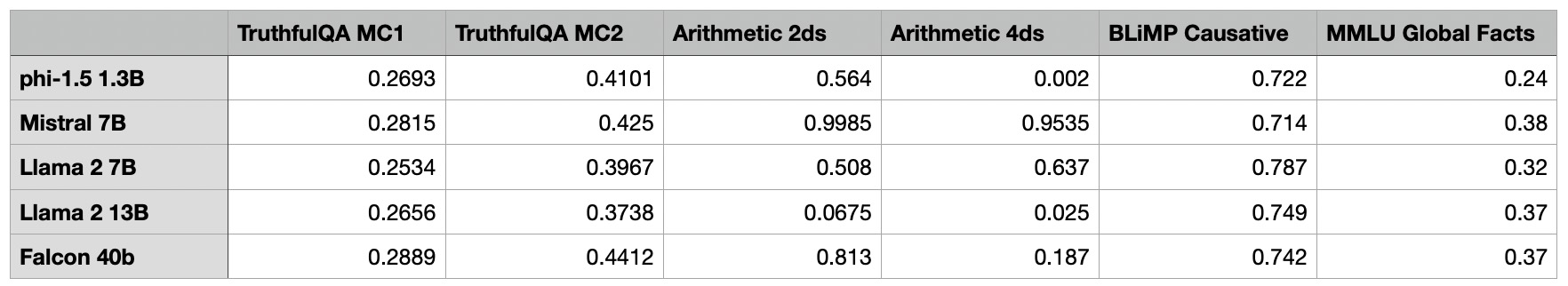
As we can see from the table above, the Mistral 7B model performs extraordinarily well on the math benchmarks. Meanwhile, the phi-1.5 1.3B model showcases impressive TruthfulQA MC2 performance given its relatively small size. For some reason, Llama 2 13B struggles with the arithmetic benchmarks, whereas the smaller Llama 2 7B outperforms it significantly in that area.

Since researchers and practitioners are currently speculating that phi-1.5 1.3B and Mistral 7B might have been trained on benchmark test data, I chose not to use them in my experiments. Moreover, I believed that selecting the smallest of the remaining models would provide the most room for improvement while maintaining lower hardware requirements. Therefore, the remainder of this article will focus on Llama 2 7B.

Evaluating the LoRA Defaults

First, I evaluated LoRA finetuning with the following default settings (these can be changed in the finetune/lora.py script):

# Hyperparameters
learning_rate = 3e-4
batch_size = 128
micro_batch_size = 1
max_iters = 50000  # train dataset size
weight_decay = 0.01
lora_r = 8
lora_alpha = 16
lora_dropout = 0.05
lora_query = True
lora_key = False
lora_value = True
lora_projection = False
lora_mlp = False
lora_head = False
warmup_steps = 100

(Note that the batch size is 128, but we are using gradient accumulation with a microbatch size of 1 to save memory; it results in the equivalent training trajectory as regular training with batch size 128. If you are curious about how gradient accumulation works, please see my article Finetuning LLMs on a Single GPU Using Gradient Accumulation).

This configuration trained 4,194,304 LoRA parameters out of a total of 6,738,415,616 trainable parameters and took approximately 1.8 hours on my machine using a single A100. The maximum memory usage was 21.33 GB.

To gauge the variance, I repeated the experiment three times to observe the fluctuation in performance between runs.

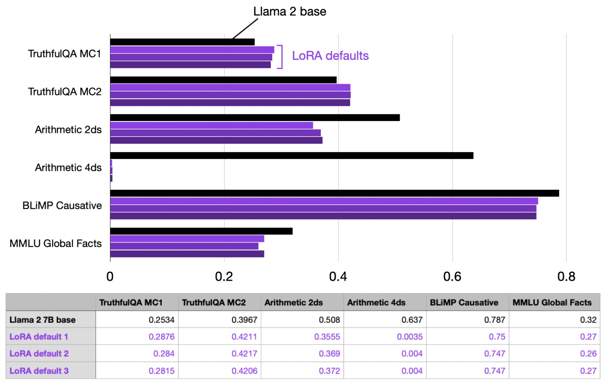
As we can see in the table above, the performance between runs is very consistent and stable. It’s also worth noting that the LoRA default model became really bad at arithmetic, but this is probably to be expected as Alpaca does not contain (m)any arithmetic tasks to the best of my knowledge.

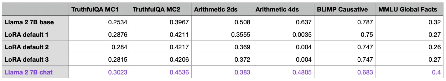
In addition, I also looked at the 7B Llama 2 version that has been instruction-finetuned by Meta using RLHF. As we can see based on the table below, the arithmetic performance is also worse for Meta’s Llama 2 Chat model as well. However, the Chat model is much improved on the other benchmarks (except BLiMP), which we can use as a reference that we want to approach with LoRA finetuning.

Memory Savings with QLoRA

Before we start tuning the LoRA hyperparameters, I wanted to explore the trade-off between modeling performance and memory savings provided by QLoRA (the popular quantized LoRA technique by Dettmers et al). 

We can enable QLoRA via the –quantize flag (here with 4-bit Normal Float type) in Lit-GPT as follows:

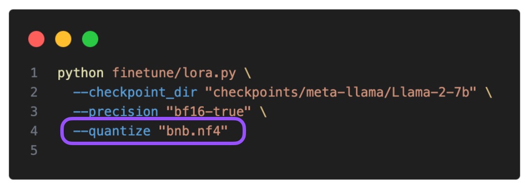
In addition, I also tried 4-bit floating point precision as a control. Below is the impact on the training time and maximum memory usage:

Default LoRA (with bfloat-16):

• Training time: 6685.75s
• Memory used: 21.33 GB

QLoRA via –-quantize “bnb.nf4”:

• Training time: 10059.53s
• Memory used: 14.18 GB

QLoRA via –quantize “bnb.fp4”:

• Training time: 9334.45s
• Memory used: 14.19 GB

We can see that QLoRA decreases the memory requirements by almost 6 GB. However, the tradeoff is a 30% slower training time, which is to be expected due to the additional quantization and dequantization steps.

Next, let’s take a look at how QLoRA training affects the model performance:

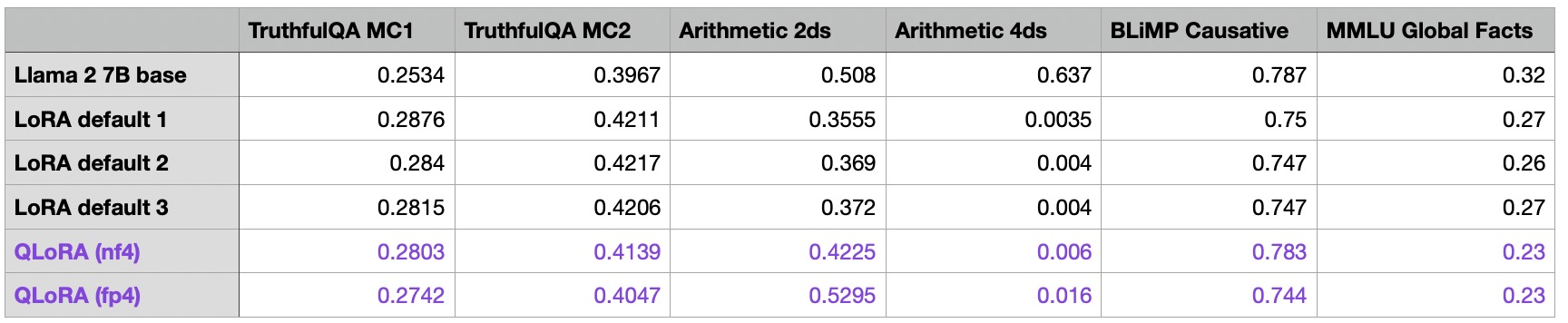
As we can see in the table above, QLoRA does have a small impact on the model performance compared to regular QLoRA. The model improves on the arithmetic benchmarks but declines on the MMLU Global Facts benchmark. 

Since the memory savings are quite substantial (which usually outweighs the longer training time since it allows users to run the models on smaller GPUs), I will use QLoRA for the remainder of the article.

Learning Rate Schedulers and SGD

I used the AdamW optimizer for all the previous experiments since it’s a common choice for LLM training. However, it’s well known that the Adam optimizer can be quite memory-intensive. This is because it introduces and tracks two additional parameters (the moments m and v) for each model parameter. Large language models (LLMs) have many model parameters; for instance, our Llama 2 model has 7 billion model parameters.

This section explores whether it’s worthwhile swapping AdamW with an SGD optimizer. However, for SGD optimizers it’s especially important to also introduce a learning rate scheduler. I opted for a cosine annealing schedule that lowers the learning rate after each batch update.

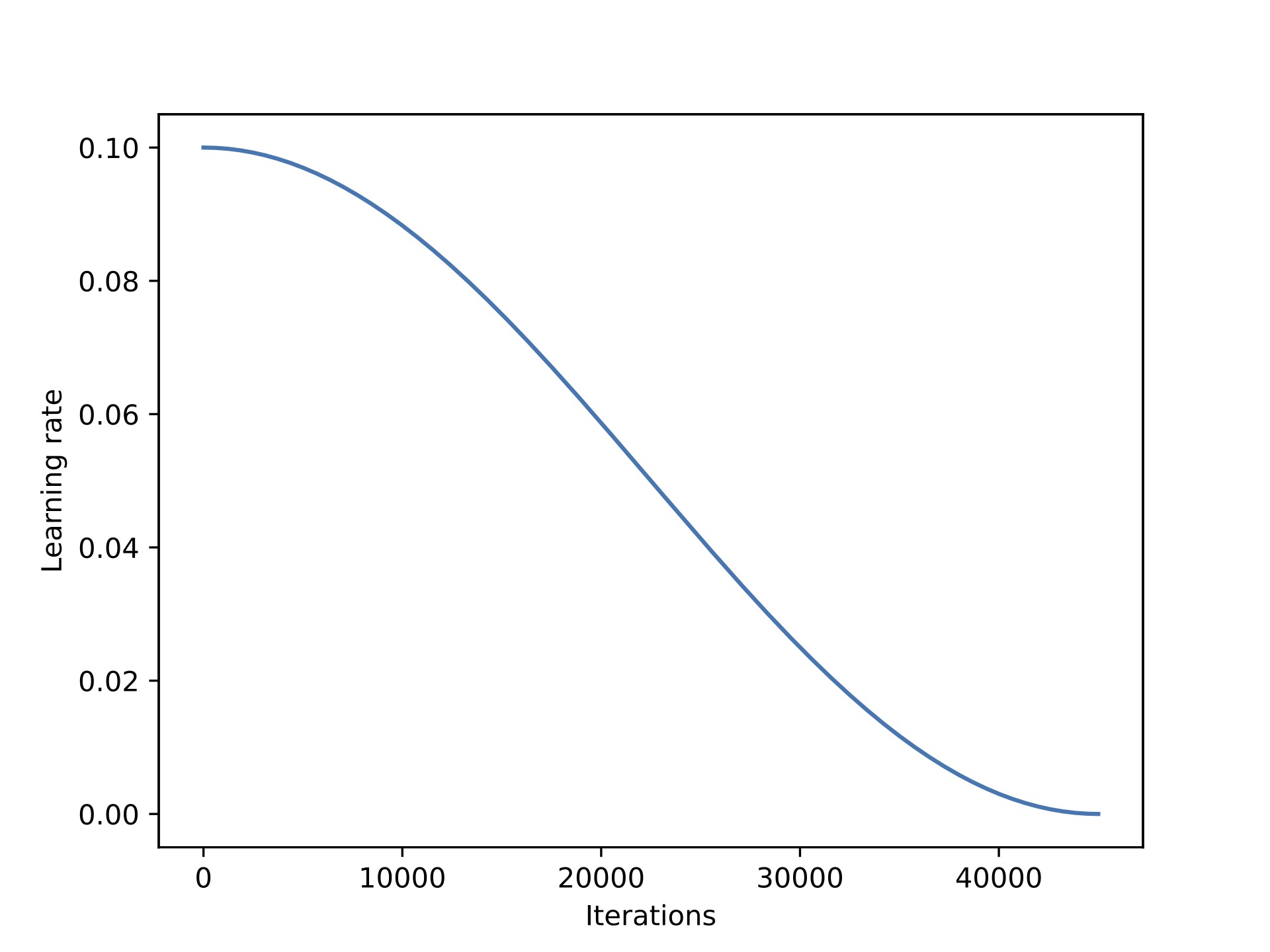
If you are interested in more details on using learning rate schedulers in PyTorch, I have a lecture on it here.

Unfortunately, swapping AdamW with SGD resulted in only minor memory savings.

• AdamW: 14.18 GB
• SGD: 14.15 GB

This is likely due to the fact that the most memory is spend on large matrix multiplications rather than keeping additional parameters in memory.

But this small difference is perhaps expected. With the currently chosen LoRA configuration (r=8), we have 4,194,304 trainable parameters. If Adam adds 2 additional values for each model parameter, which are stored in 16-bit floats, we have 4,194,304 * 2 * 16 bit = 134.22 megabits = 16.78 megabytes.

We can observe a larger difference when we increase LoRA’s r to 256, which we will do later. In the case of r=256, we have 648,871,936 trainable parameters, which equals 2.6 GB using the same calculation as above. The actual measurement resulted in a 3.4 GB difference, perhaps due to some additional overhead in storing and copying optimizer states.

The bottom line is that for small numbers of trainable parameters, such as in the case with LoRA and low r (rank) values, the memory gain from swapping AdamW with SGD can be very small, in contrast to pretraining, where we train a larger number of parameters.

Even though SGD does not provide us with notable memory savings here, let’s still have a quick look at the resulting model performance:

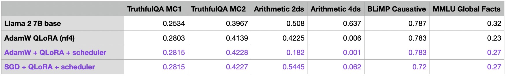
It seems that the performance of the SGD optimizer is comparable to that of AdamW. Interestingly, when a scheduler is added to AdamW, there’s an improvement in the TruthfulQA MC2 and MMLU Global Facts performances, but a decrease in arithmetic performance. (Note: TruthfulQA MC2 is a widely recognized benchmark featured in other public leaderboards.) For the time being, we won’t place too much emphasis on the arithmetic performance and will proceed with the remaining experiments in this article using AdamW with a scheduler.

If you want to reproduce these experiments, I found that the best AdamW learning rate was 3e-4 with a decay rate of 0.01. The best SGD learning rate was 0.1, with a momentum of 0.9. I used an additional 100 steps of learning rate warmup in both cases.

(Based on these experiments, the cosine scheduler has been added to Lit-GPT and is now enabled by default.)

Iterating Over the Dataset Multiple Times

So far, I have trained all models with 50k iterations — the Alpaca dataset has 50k training examples. The obvious question is whether we can improve the model performance by iterating over the training set multiple times, so I ran the previous experiment with 100k iterations, which is a 2-fold increase:

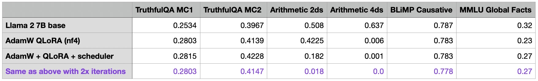
Interestingly, the increased iterations result in worse performance across the board. The decline is most significant for the arithmetic benchmarks. My hypothesis is that the Alpaca dataset does not contain any related arithmetic tasks, and the model actively unlearns basic arithmetic when it focuses more on other tasks.

Anyway, I would be lying if I said this outcome wasn’t welcome. This way, I can continue with the shorter 50k iteration experiments for the remainder of this article.

LoRA Hyperparameter Tuning Part 1: LoRA for All Layers

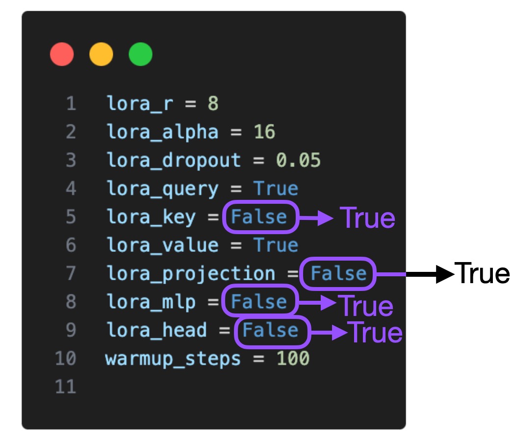
Now that we have explored the basic settings surrounding the LoRA finetuning scripts, let’s turn our attention to the LoRA hyperparameters themselves. By default, LoRA was only enabled for the Key and Query matrices in the multi-head self-attention blocks. Now, we are also enabling it for the Value matrix, the projection layers, and the linear layers:

LoRA Hyperparameter Tuning Part 2: Increasing R

One of the most important LoRA parameters is “r”, which determines the rank or dimension of the LoRA matrices, directly influencing the complexity and capacity of the model. A higher “r” means more expressive power but can lead to overfitting, while a lower “r” can reduce overfitting at the expense of expressiveness. Keeping LoRA enabled for all layers, let’s increase the r from 8 to 16 and see what impact this has on the performance: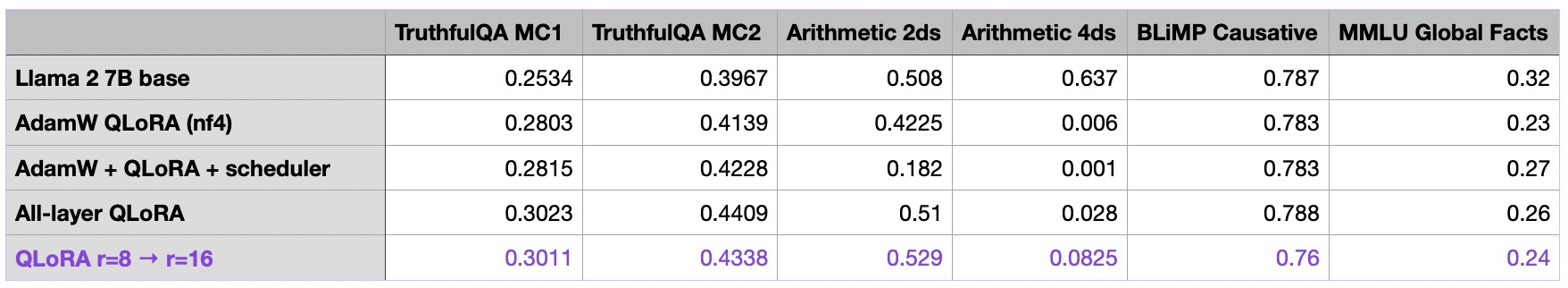

We can see that just increasing r by itself made the results worse, so what happened? Let’s find out in the next section.

LoRA Hyperparameter Tuning Part 3: Changing Alpha

In the previous section, we increase the matrix rank r while leaving LoRA’s alpha parameter unchanged. A higher “alpha” would place more emphasis on the low-rank structure or regularization, while a lower “alpha” would reduce its influence, making the model rely more on the original parameters. Adjusting “alpha” helps in striking a balance between fitting the data and preventing overfitting by regularizing the model.

As a rule of thumb, it’s usually common to choose an alpha that is twice as large as the rank when finetuning LLMs (note that this is different when working with diffusion models). Let’s try this out and see what happens when we increase alpha two-fold:

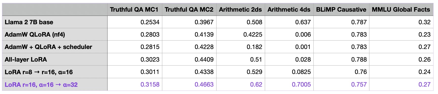
As we can see, increasing alpha to 32 now yields our best model thus far! But again we bought  this improvement with a larger number of parameters to be trained:

r=8:

• Number of trainable parameters: 20,277,248
• Number of non trainable parameters: 6,738,415,616
• Memory used: 16.42 GB

r=16:

• Number of trainable parameters: 40,554,496
• Number of non trainable parameters: 6,738,415,616
• Memory used: 16.47 GB

However, the number of trainable parameters is still small enough that it doesn’t noticeably impact the peak memory requirements.

Anyways, we are now finally starting to make some gains and improve the model performance by more noticeable margins. So, let’s keep going and see how far we can push this by increasing the rank and alpha:

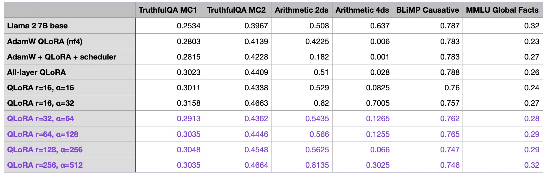
I also ran additional experiments with exceptionally large ranks (512, 1024, and 2048), but these resulted in poorer outcomes. Some of the runs didn’t even converge to a near-zero loss during training, which is why I didn’t add them to the table.

So far, we can note that the r=256 and alpha=512 model in the last row resulting in the best performance overall so far. As an additional control experiments, I repeated the runs with an alpha of 1 and noticed that a large alpha value was indeed necessary for the good performance:

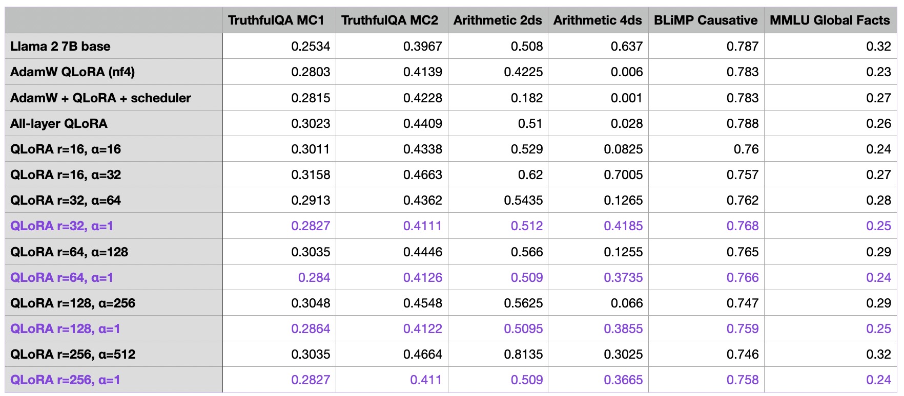
I also repeated the experiments with alpha values of 16 and 32, and I observed the same worse performance compared to choosing the alpha value as two-times the rank.

LoRA Hyperparameter Tuning Part 3: Very Large R

For the final tuning experiment of this article, I wanted to further optimize the alpha value of the best model from the previous section (r=256, last row), suspecting that it might be a bit too large.

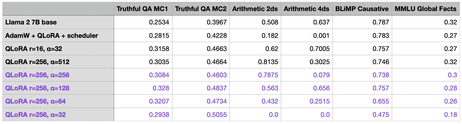
As seen in the table above, choosing a large alpha value appears to be crucial when increasing the rank.

For the QLoRA model with r=256 and a=512, it’s evident that our model has made significant improvements over the base model. The only area where the finetuned model underperforms compared to the base model is in 4-digit arithmetic. However, this is understandable, considering the Alpaca dataset probably did not contain such training examples.

Above, we’ve seen that the common recommendation of choosing alpha as two-times the rank (e.g., r=256 and alpha=512) indeed yielded the best results, and smaller alpha values resulted in worse outcomes. But how about increasing alpha past the “two-fold the rank” recommendation?

Based on the results provided in the table above, choosing alpha such that it exceeds the “two-fold the rank” recommendation also makes the benchmark outcomes worse.

Leaderboard Submission

We know that in machine learning, we should not use the test set multiple times. Otherwise, we risk over-optimizing to a specific task. Hence, it’s recommended to validate a model on a final independent dataset.

Coincidentally, there’s currently the NeurIPS LLM Efficiency challenge under way, which is focused on finetuning an LLM on a single GPU. Since I was curious to see how the Llama-2 7B base model compares to our best LoRA model finetuned on Alpaca, I submitted both the base and the finetune model to their leaderboard.

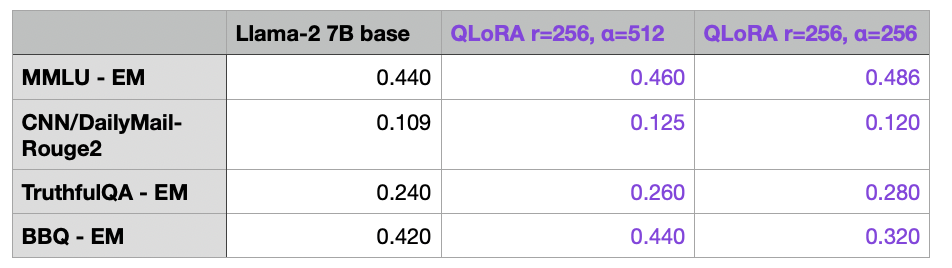
We can see that the (Q)LoRA finetuning, which took 10522.77s (~3h) to train and required 19.24 GB GPU memory with the r=256 setting, improved the performance on several but not all benchmarks. The performance could potentially be improved by considering different finetuning datasets other than Alpaca and considering alignment techniques such as RLHF, which I explained in more detail here.

Conclusion

This article explored the various knobs we can tune when training custom LLMs using LoRA. We found that QLoRA is a great memory-saver even though it comes at an increased runtime cost. Moreover, while learning rate schedulers can be beneficial, choosing between AdamW and SGD optimizers makes little difference. And iterating over the dataset more than once can make the results even worse. The best bang for the buck can be achieved by optimizing the LoRA settings, including the rank. Increasing the rank will result in more trainable parameters, which could lead to higher degrees of overfitting and runtime costs. However, when increasing the rank, choosing the appropriate alpha value is important. 

This article was by no means exhaustive and in the sense that I did not have the time and resources to explore all possible configurations. Also, future improvements could be achieved by considering other datasets and models.

I hope that you can gain one or the other insight that you can apply to your projects. I kept the background information and explanations on various concepts like LoRA, learning rate schedulers, gradient accumulation, and so on to a minimum so that this article doesn’t not become unreasonably longer. However, I am more than happy to chat if you have any questions or concerns. You can reach me on X/Twitter or LinkedIn or reach out to @LightningAI.

If you found this article useful, I would appreciate it if you could share it with your colleagues.

For general feedback, suggestions, or improvements to Lit-GPT, please feel free to use the GitHub issue tracker.