Understanding Parameter-Efficient Finetuning of Large Language Models: From Prefix Tuning to LLaMA-Adapters

In the rapidly evolving field of artificial intelligence, utilizing large language models in an efficient and effective manner has become increasingly important.

Parameter-efficient finetuning stands at the forefront of this pursuit, allowing researchers and practitioners to reuse pretrained models while minimizing their computational and resource footprints. It also allows us to train AI models on a broader range of hardware, including devices with limited computational power, such as laptops, smartphones, and IoT devices. Lastly, with the increasing focus on environmental sustainability, parameter-efficient finetuning reduces the energy consumption and carbon footprint associated with training large-scale AI models.

This article explains the broad concept of finetuning and discusses popular parameter-efficient alternatives like prefix tuning and adapters. Finally, we will look at the recent LLaMA-Adapter method and see how we can use it in practice.

Finetuning Large Language Models

Since GPT-2 (Radford et al.) and GPT-3 (Brown et al.), we have seen that generative large language models (LLMs) pretrained on a general text corpus are capable of in-context learning, which doesn’t require us to further train or finetune pretrained LLMs if we want to perform specific or new tasks that the LLM wasn’t explicitly trained on. Instead, we can directly provide a few examples of a target task via the input prompt, as illustrated in the example below.

In-context learning is a valuable and user-friendly method for situations where direct access to the large language model (LLM) is limited, such as when interacting with the LLM through an API or user interface.
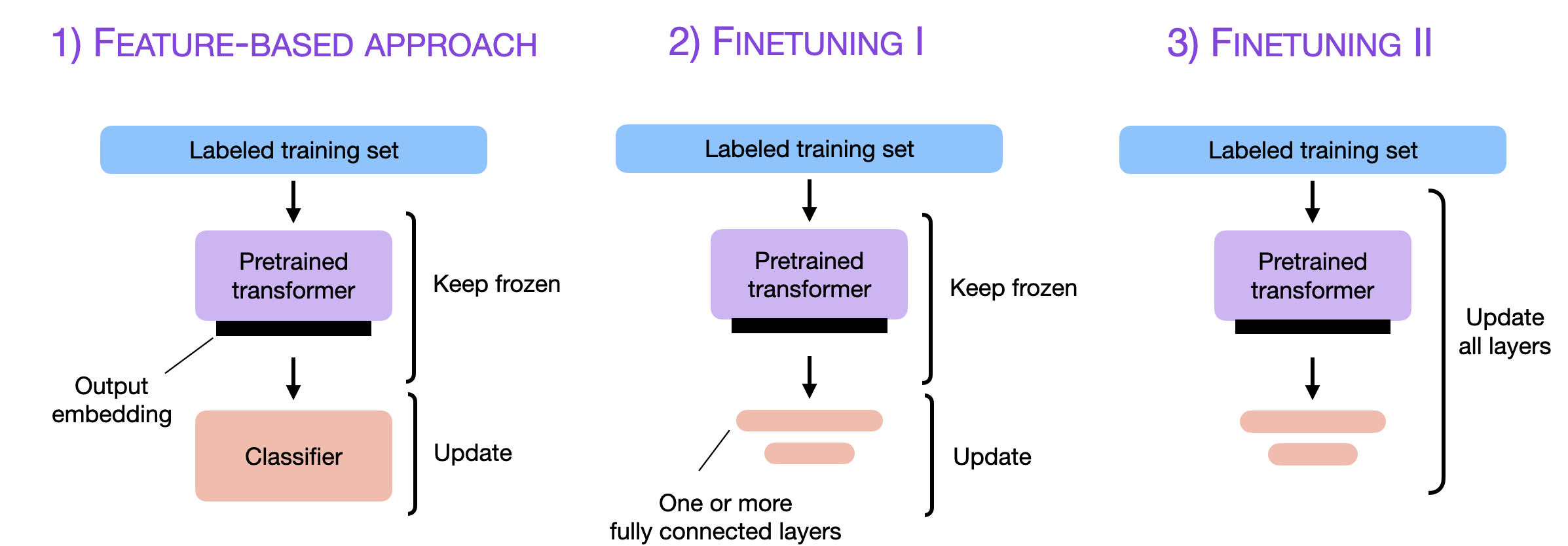
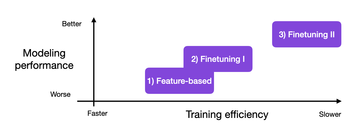
However, if we have access to the LLM, adapting and finetuning it on a target task using data from a target domain usually leads to superior results. So, how can we adapt a model to a target task? There are three conventional approaches outlined in the figure below.

These methods above are compatible with generative (decoder-style) models such as GPT and embedding-focused (encoder-style) models such as BERT. In contrast to these three approaches, in-context learning only applies to generative models. It’s also worth highlighting that when we finetune generative models, we work with and build on the embeddings they create instead of the generated output texts.

 
Feature-based approach

In the feature-based approach, we load a pretrained LLM and apply it to our target dataset. Here, we are particularly interested in generating the output embeddings for the training set, which we can use as input features to train a classification model. While this approach is particularly common for embedding-focused like BERT, we can also extract embeddings from generative GPT-style models (you can find an example in our blog post here).

The classification model can then be a logistic regression model, a random forest, or XGBoost — whatever our hearts desire. (However, based on my experience, linear classifiers like logistic regression perform best here.)

Conceptually, we can illustrate the feature-based approach with the following code:

model = AutoModel.from_pretrained("distilbert-base-uncased")

# ...

# tokenize dataset

# ...

# generate embeddings

@torch.inference_mode()

def get_output_embeddings(batch):

    output = model(

        batch["input_ids"],

        attention_mask=batch["attention_mask"]

    ).last_hidden_state[:, 0]

return {"features": output}

dataset_features = dataset_tokenized.map(

  get_output_embeddings, batched=True, batch_size=10)

X_train = np.array(dataset_features["train"]["features"])

y_train = np.array(dataset_features["train"]["label"])

X_val = np.array(dataset_features["validation"]["features"])

y_val = np.array(dataset_features["validation"]["label"])

X_test = np.array(dataset_features["test"]["features"])

y_test = np.array(dataset_features["test"]["label"])

# train classifier

from sklearn.linear_model import LogisticRegression

clf = LogisticRegression()

clf.fit(X_train, y_train)

print("Training accuracy", clf.score(X_train, y_train))

print("Validation accuracy", clf.score(X_val, y_val))

print("test accuracy", clf.score(X_test, y_test))

ExpandCopy

(Interested readers can find the full code example here.)

 
Finetuning I — Updating The Output Layers

A popular approach related to the feature-based approach described above is finetuning the output layers (we will refer to this approach as finetuning I). Similar to the feature-based approach, we keep the parameters of the pretrained LLM frozen. We only train the newly added output layers, analogous to training a logistic regression classifier or small multilayer perceptron on the embedded features.

In code, this would look as follows:

model = AutoModelForSequenceClassification.from_pretrained(

    "distilbert-base-uncased",

     num_labels=2  # suppose target task is a binary classification task

) 

# freeze all layers

for param in model.parameters():

    param.requires_grad = False

# then unfreeze the two last layers (output layers)

for param in model.pre_classifier.parameters():

    param.requires_grad = True

for param in model.classifier.parameters():

    param.requires_grad = True

# finetune model

lightning_model = CustomLightningModule(model)

trainer = L.Trainer(

    max_epochs=3,

    ...

)

trainer.fit(

  model=lightning_model,

  train_dataloaders=train_loader,

  val_dataloaders=val_loader)

# evaluate model

trainer.test(lightning_model, dataloaders=test_loader)

ExpandCopy

(Interested readers can find the complete code example here.)

In theory, this approach should perform similarly well, in terms of modeling performance and speed, as the feature-based approach since we use the same frozen backbone model. However, since the feature-based approach makes it slightly easier to pre-compute and store the embedded features for the training dataset, the feature-based approach may be more convenient for specific practical scenarios.

 
Finetuning II — Updating All Layers

While the original BERT paper (Devlin et al.) reported that finetuning only the output layer can result in modeling performance comparable to finetuning all layers, which is substantially more expensive since more parameters are involved. For instance, a BERT base model has approximately 110 million parameters. However, the final layer of a BERT base model for binary classification consists of merely 1,500 parameters. Furthermore, the last two layers of a BERT base model account for 60,000 parameters — that’s only around 0.6% of the total model size.

Our mileage will vary based on how similar our target task and target domain is to the dataset the model was pretrained on. But in practice, finetuning all layers almost always results in superior modeling performance.

So, when optimizing the modeling performance, the gold standard for using pretrained LLMs is to update all layers (here referred to as finetuning II). Conceptually finetuning II is very similar to finetuning I. The only difference is that we do not freeze the parameters of the pretrained LLM but finetune them as well:

model = AutoModelForSequenceClassification.from_pretrained(

    "distilbert-base-uncased",

     num_labels=2  # suppose target task is a binary classification task

) 

# don't freeze layers

# for param in model.parameters():

#    param.requires_grad = False

# finetune model

lightning_model = LightningModel(model)

trainer = L.Trainer(

    max_epochs=3,

    ...

)

trainer.fit(

  model=lightning_model,

  train_dataloaders=train_loader,

  val_dataloaders=val_loader)

# evaluate model

trainer.test(lightning_model, dataloaders=test_loader)

ExpandCopy

(Interested readers can find the complete code example here.)

If you are curious about some real-world results, the code snippets above were used to train a movie review classifier using a pretrained DistilBERT base model (you can access the code notebooks here):
Feature-based approach with logistic regression: 83% test accuracy
Finetuning I, updating the last 2 layers: 87% accuracy
Finetuning II, updating all layers: 92% accuracy.
These results are consistent with the general rule of thumb that finetuning more layers often results in better performance, but it comes with increased cost.

Parameter-Efficient Finetuning

In the previous sections, we learned that finetuning more layers usually leads to better results. Now, the experiments above are based on a DistilBERT model, which is relatively small. What if we want to finetune larger models that only barely fit into GPU memory, for example, the latest generative LLMs? We can use the feature-based or finetuning I approach above, of course. But suppose we want to get a similar modeling quality as finetuning II?

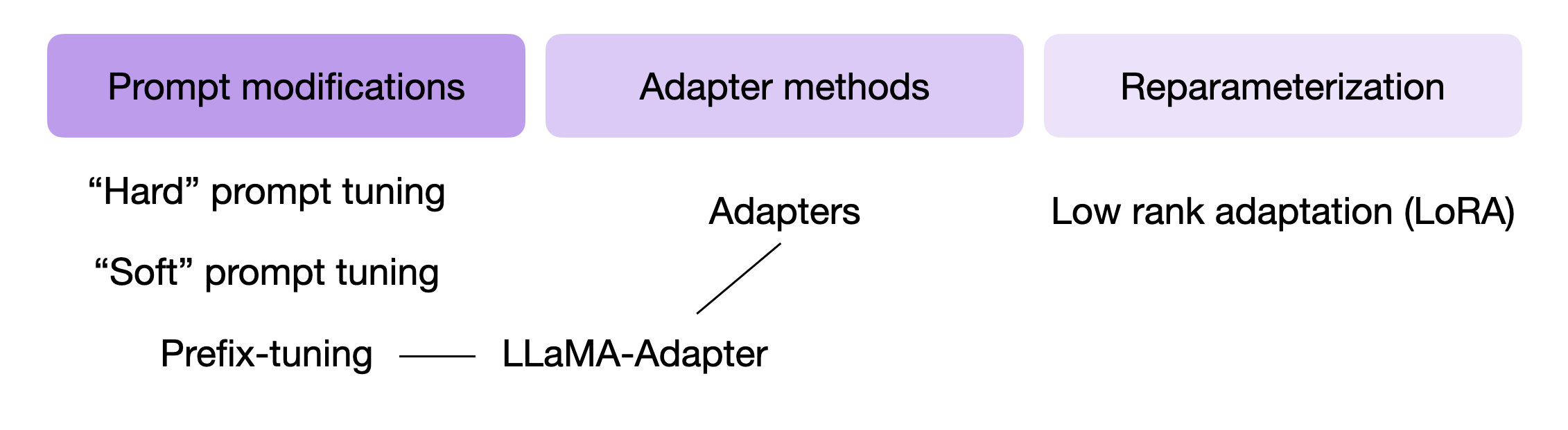
Over the years, researchers developed several techniques (Lialin et al.) to finetune LLM with high modeling performance while only requiring the training of only a small number of parameters. These methods are usually referred to as parameter-efficient finetuning techniques (PEFT).

Some of the most widely used PEFT techniques are summarized in the figure below.

One PEFT technique that recently made big waves is LLaMA-Adapter, which was proposed for Meta’s popular LLaMA model (Touvron et al.) — however, while LLaMA-Adapter was proposed in the context of LLaMA, the idea is model-agnostic.

To understand how LLaMA-Adapter works, we have to take a (small) step back and review two related techniques called prefix tuning and adapters — LLaMA-Adapter (Zhang et al.) combines and extends both of these ideas.

So, in the remainder of this article, we will discuss the various concepts of prompt modifications to understand prefix tuning and adapter methods before we take a closer look at LLaMA-Adapter. (And we will save low-rank adaptation for a future article.)

Prompt Tuning And Prefix Tuning

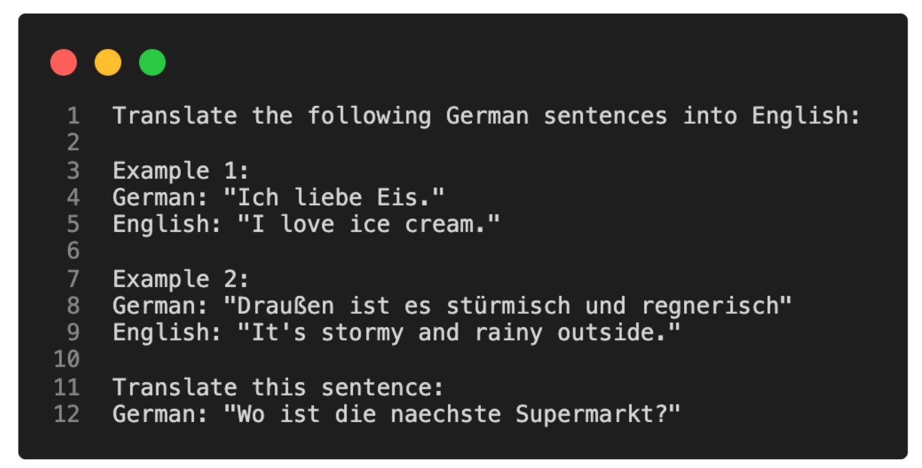
The original concept of prompt tuning refers to techniques that vary the input prompt to achieve better modeling results. For example, suppose we are interested in translating an English sentence into German. We can ask the model in various different ways, as illustrated below.

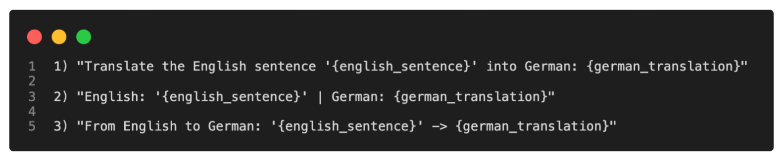
Now, this concept illustrated above is referred to as hard prompt tuning since we directly change the discrete input tokens, which are not differentiable. 

In contrast to hard prompt tuning, soft prompt tuning concatenates the embeddings of the input tokens with a trainable tensor that can be optimized via backpropagation to improve the modeling performance on a target task. 

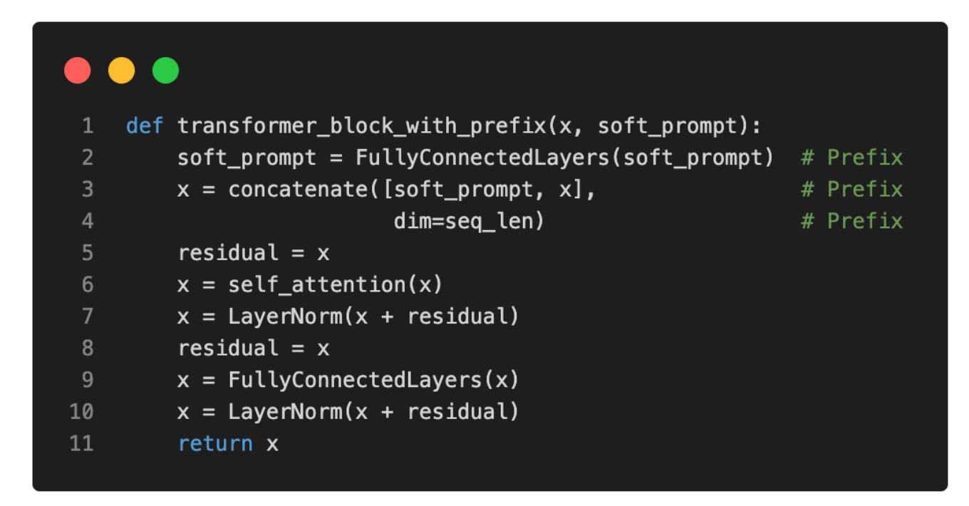
A specific flavor of prompt tuning is prefix tuning (Li and Liang). The idea in prefix tuning is to add a trainable tensor to each transformer block instead of only the input embeddings, as in soft prompt tuning. The following figure illustrates the difference between a regular transformer block and a transformer block modified with a prefix.

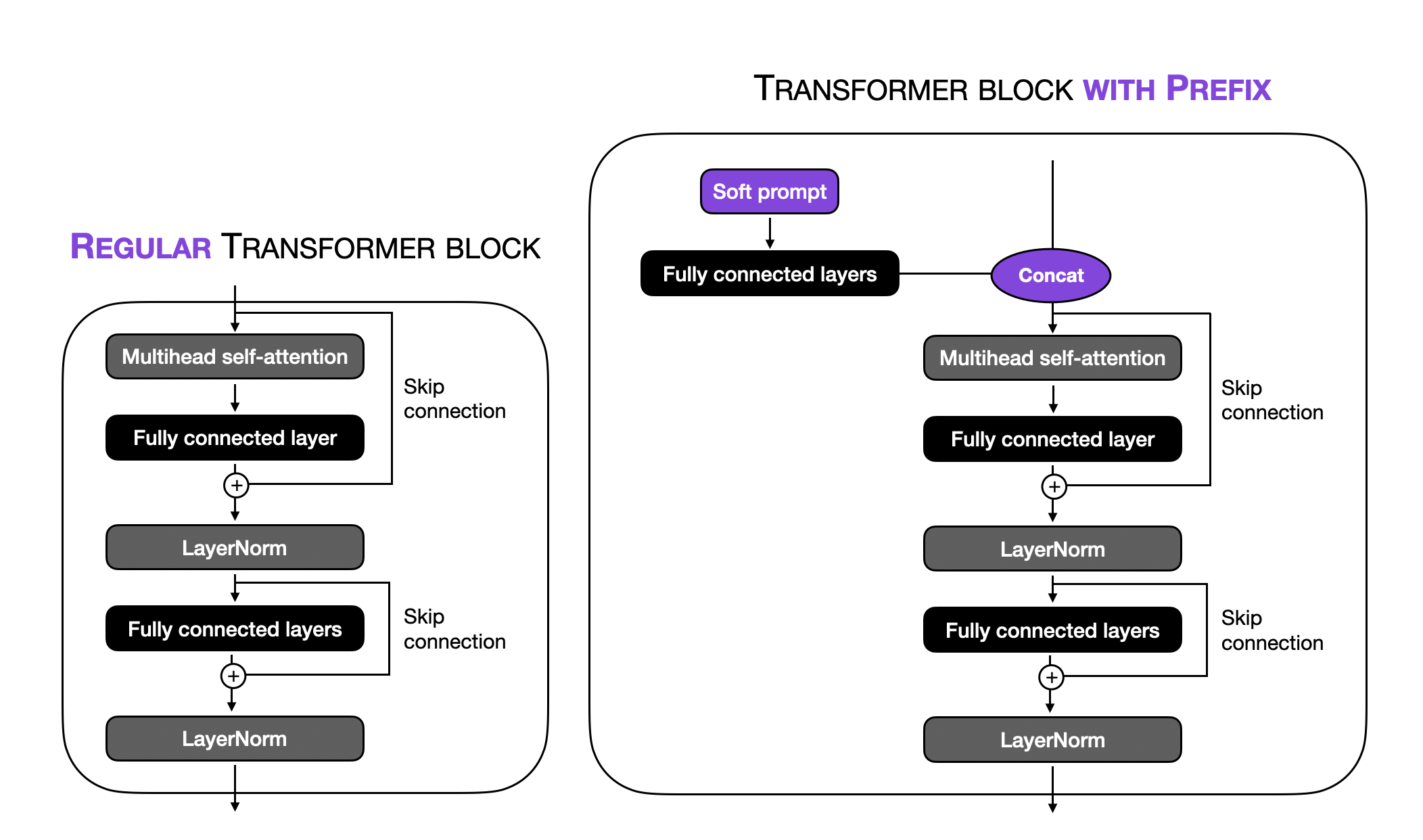
Note that in the figure above, the “fully connected layers” refer to a small multilayer perceptron (two fully connected layers with a nonlinear activation function in-between). These fully connected layers embed the soft prompt in a feature space with the same dimensionality as the transformer-block input to ensure compatibility for concatenation.
Using (Python) pseudo-code, we can illustrate the difference between a regular transformer block and a prefix-modified transformer block as follows:

According to the original prefix tuning paper, prefix tuning achieves comparable modeling performance to finetuning all layers while only requiring the training of 0.1% of the parameters — the experiments were based on GPT-2 models. Moreover, in many cases, prefix tuning even outperformed the finetuning of all layers, which is likely because fewer parameters are involved, which helps reduce overfitting on smaller target datasets.

Lastly, to clarify the use of soft prompts during inference: after learning a soft prompt, we have to supply it as a prefix when performing the specific task we finetuned the model on. This allows the model to tailor its responses to that particular task. Moreover, we can have multiple soft prompts, each corresponding to a different task, and provide the appropriate prefix during inference to achieve optimal results for a particular task.

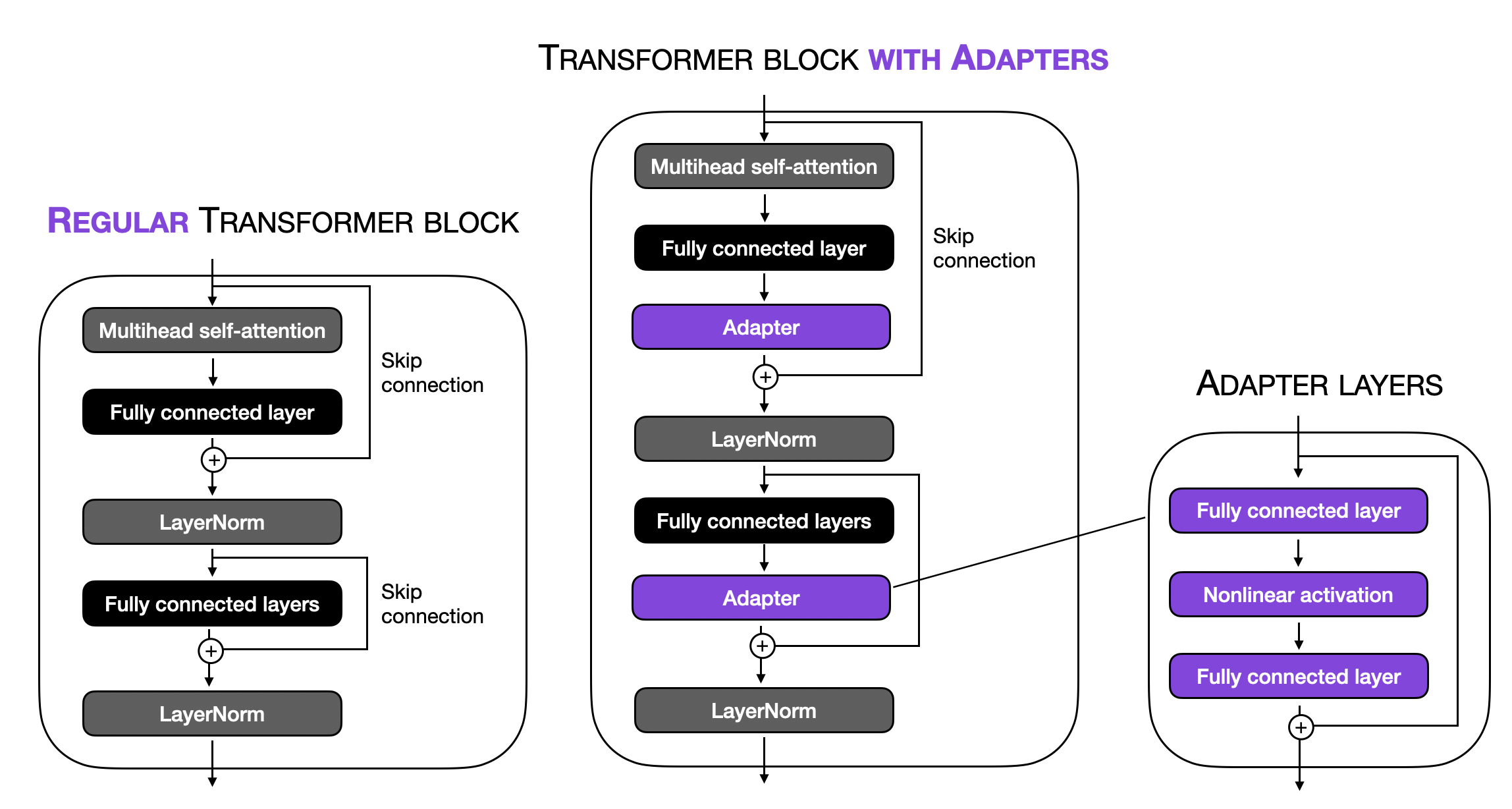
Adapters

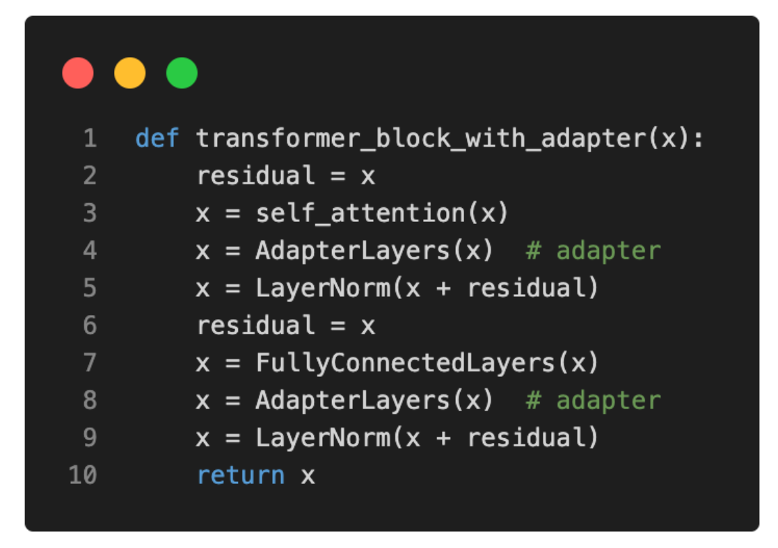
The original adapter method (Houlsby et al.) is somewhat related to the aforementioned prefix tuning as they also add additional parameters to each transformer block. However, instead of prepending prefixes to the input embeddings, the adapter method adds adapter layers in two places, as illustrated in the figure below.

And for readers who prefer (Python) pseudo-code, the adapter layer can be written as follows:

Note that the fully connected layers of the adapters are usually relatively small and have a bottleneck structure similar to autoencoders. Each adapter block’s first fully connected layer projects the input down onto a low-dimensional representation. The second fully connected layer projects the input back into the input dimension. How is this parameter efficient? For example, assume the first fully connected layer projects a 1024-dimensional input down to 24 dimensions, and the second fully connected layer projects it back into 1024 dimensions. This means we introduced 1,024 x 24 + 24 x 1,024 = 49,152 weight parameters. In contrast, a single fully connected layer that reprojects a 1024-dimensional input into a 1,024-dimensional space would have 1,024 x 1024 = 1,048,576 parameters.

According to the original adapter paper, a BERT model trained with the adapter method reaches a modeling performance comparable to a fully finetuned BERT model while only requiring the training of 3.6% of the parameters.

Now, the question is how the adapter method compares to prefix tuning. Based on the original prefix tuning paper, the adapter method performed slightly worse than the prefix tuning method when 0.1% of the total number of model parameters were tuned. However, when the adapter method is used to tune 3% of the model parameters, the method ties with prefix tuning of 0.1% of the model parameters. So, we may conclude that the prefix tuning method is the more efficient of the two.

Extending Prefix Tuning and Adapters: LLaMA-Adapter

Extending the ideas of prefix tuning and the original adapter method, researchers recently proposed LLaMA-Adapter (Zhang et al.), a parameter-efficient finetuning method for LLaMA (LLaMA is a popular GPT-alternative by Meta).

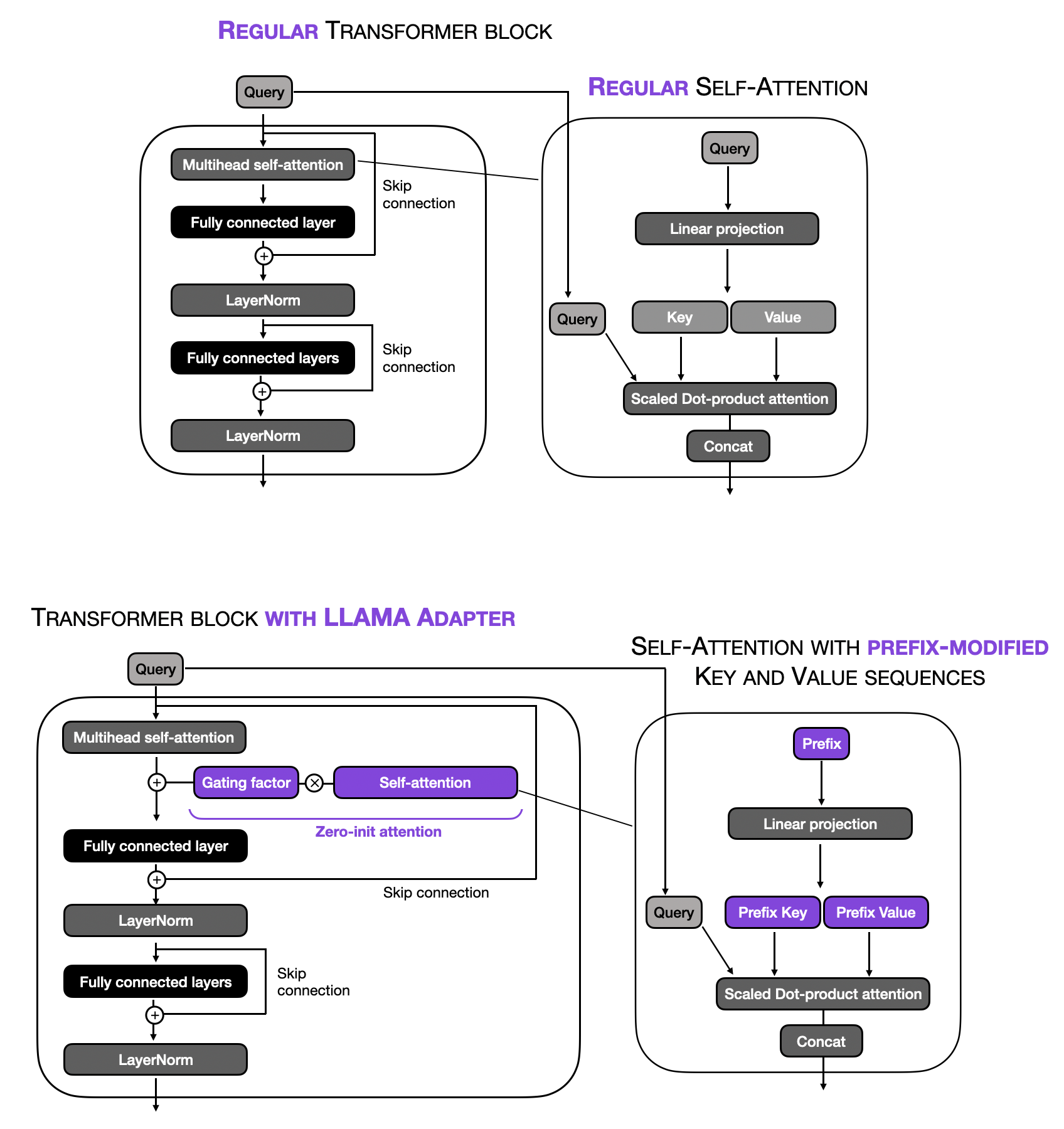
Like prefix tuning, the LLaMA-Adapter method prepends tunable prompt tensors to the embedded inputs. It’s worth noting that in the LLaMA-Adapter method, the prefix is learned and maintained within an embedding table rather than being provided externally. Each transformer block in the model has its own distinct learned prefix, allowing for more tailored adaptation across different model layers.

In addition, LLaMA-Adapter introduces a zero-initialized attention mechanism coupled with gating. The motivation behind this so-called zero-init attention and gating is that adapters and prefix tuning could potentially disrupt the linguistic knowledge of the pretrained LLM by incorporating randomly initialized tensors (prefix prompts or adapter layers), resulting in unstable finetuning and high loss values during initial training phases.

Another difference compared to prefix tuning and the original adapter method is that LLaMA-Adapter adds the learnable adaption prompts only to the L topmost transformer layers instead of all transformer layers. The authors argue that this approach enables more effective tuning of language representations focusing on higher-level semantic information.

While the basic idea of the LLaMA adapter method is related to prefix tuning (prepending tunable soft prompts), there are some additional, subtle differences in how this is implemented. For instance, only a self-attention input’s key and value sequences are modified via the tunable soft prompt. Then, depending on the gating factor (which is set to zero at the beginning of the training), the prefix-modified attention is either used or not. This concept is illustrated in the visualization below.

In pseudo-code, we may express this as follows:

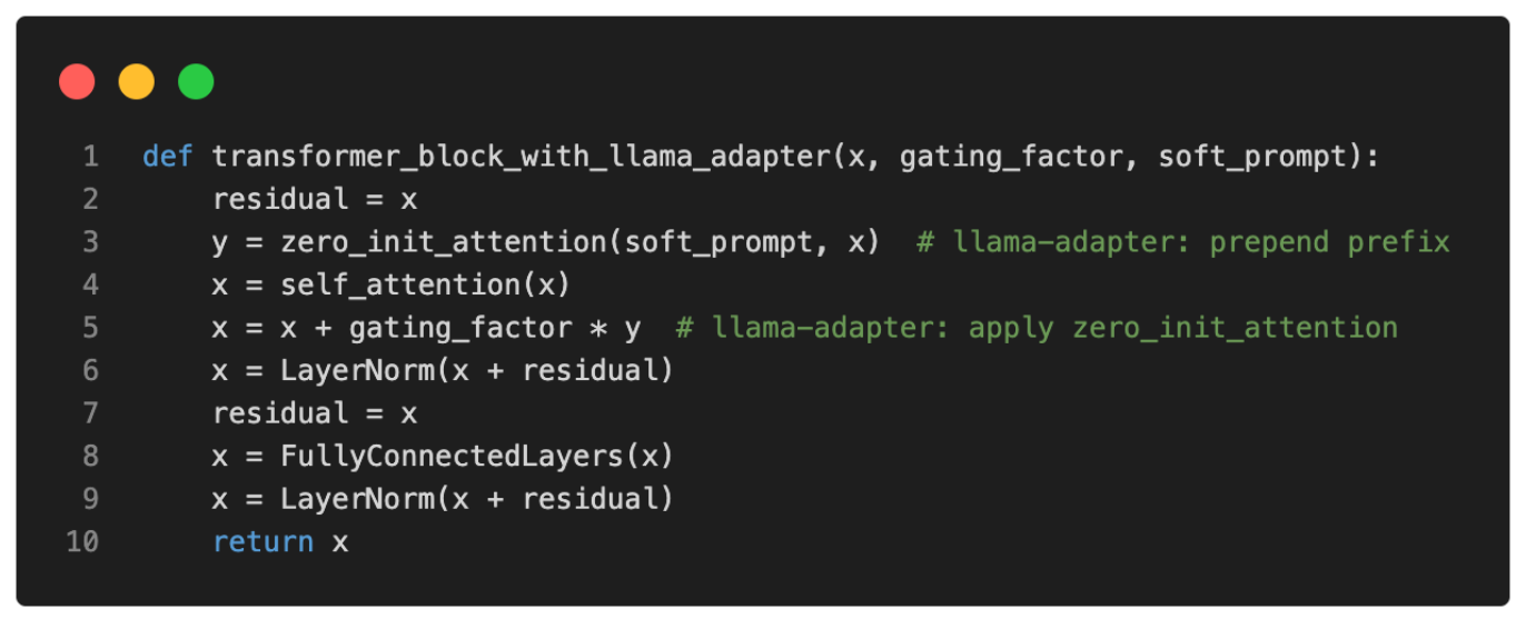
In short, the differences between LLaMA-Adapter and regular prefix tuning are that LLaMA-Adapter only modifies the top (i.e., the first few) transformer blocks and introduces a gating mechanism to stabilize the training. While the researchers specifically experiment with LLaMA, their proposed Adapter method is a general method that can also be applied to other types of LLMs (like GPT).

Using the LLaMA-Adapter approach, the researchers were able to finetune a 7 billion parameter LLaMA model in only 1 hour (using eight A100 GPUs) on a dataset consisting of 52k instruction pairs. Furthermore, the finetuned LLaMA-Adapter model outperformed all other models compared in this study on question-answering tasks, while only 1.2 M parameters (the adapter layers) needed to be finetuned.

If you want to check out the LLaMA-Adapter method, you can find the original implementation on top of the GPL-licensed LLaMA code here.

Alternatively, if your use cases are incompatible with the GPL license, which requires you to open source all derivative works under a similar license, check out the Lit-LLaMA GitHub repository. Lit-LLaMA is a readable implementation of LLaMA on top of the Apache-licensed nanoGPT code, which has less restrictive licensing terms.

Specifically, if you are interested in finetuning a LLaMA model using the LLaMA-Apapter method, you can run the

python finetune_adapter.py

ExpandCopy

script from the Lit-LLaMA GitHub repository.

Conclusion

Finetuning pre-trained large language models (LLMs) is an effective method to tailor these models to suit specific business requirements and align them with target domain data. This process involves adjusting the model parameters using a smaller dataset relevant to the desired domain, which enables the model to learn domain-specific knowledge and vocabulary.

However, as LLMs are “large,” updating multiple layers in a transformer model can be very expensive, so researchers started developing parameter-efficient alternatives.

In this article, we discussed several parameter-efficient alternatives to the conventional LLM finetuning mechanism. In particular, we covered prepending tunable soft prompts via prefix tuning and inserting additional adapter layers.

Finally, we discussed the recent and popular LLaMA-Adapter method that prepends tunable soft prompts and introduces an additional gating mechanism to stabilize the training.

If you want to try this out in practice, check out the Lit-LLaMA repository — questions and suggestions for additional parameter-efficient finetuning methods are very welcome! (Preferably via the 🦙lit-llama channel on Discord)

Acknowledgments

I want to thank Carlos Mocholi, Luca Antiga, and Adrian Waelchli for the constructive feedback to improve the clarity of this article.