Takeaways
A generic four line code change can reduce peak memory by 20-40% when training large models.
Before
optimizer = Optimizer(model.parameters(), ...)
...
for inputs, targets in epoch:
loss = loss_fn(model(inputs), targets)
loss.backward()
optimizer.step()
optimizer.zero_grad()
After
from lightning.fabric.strategies.fsdp import fsdp_overlap_step_with_backward
optimizers = [Optimizer([p], ...) for p in model.parameters()]
...
for inputs, targets in epoch:
loss = loss_fn(model(inputs), targets)
with fsdp_overlap_step_with_backward(optimizers, model):
loss.backward()
The curse of OOM
One of the main challenges in training multi-billion parameter models is dealing with limited GPU memory while training. In fact, getting out-of-memory (OOM) errors is arguably one of the bummers of every practitioner.
During training, there are several sets of tensor data to keep in memory, which include:
- model parameters
- optimizer state
- inputs and other temporary tensors
- activations
- gradients and Autograd-related intermediates
- communication buffers
All these contribute to getting our training process running out of memory.
There is a wide selection of techniques to mitigate the problem, such as sharding parameters (and optionally gradients and optimizer state) across multiple GPUs and gathering them only when needed, or offloading them to main memory, if you’re ok with the inherent slowdown due to moving things between main memory and device memory.
One can also trade memory for speed by choosing to not retain all activations between forward and backward passes, but recomputing them when needed, like in activation checkpointing. Other approaches like model and tensor parallelism reduce memory requirements on the individual GPU by performing computations of different parts of the model across different GPUs. Finally, one can reduce memory usage by lowering precision, or adopting quantization or sparsification strategies.
What is lesser known however, is that it is not necessarily a matter of how much data we need to keep in memory during training, but when that happens. As in, do we need to keep all of the above in memory at once, or can we be smart about what we materialize and when, so that we avoid OOM’ing due to an avoidable memory spike happening at some point along the way?
In this post we will dive into this question and show that yes, it’s all about the when, and this impacts not just the amount of memory but also the throughput that we can obtain. Poorly managed memory, the need of allocating it or re-allocating it, can cause GPUs to stall for incredibly long amounts of time, and will render any other optimization we can layer on top moot.
Luckily Fabric comes to the rescue with a brand new context manager (fsdp_overlap_step_with_backward) that takes care of managing the “when” optimally for you. It does it in the tricky situation of running with an FSDP strategy, which is kind of a given since we are targeting larger models.
What’s going on?
The idiomatic way of writing PyTorch code breaks a training step into discrete steps.
...
loss = loss_fn(model(inputs, targets)) # store activations
loss.backward() # compute all gradients
optimizer.step() # apply parameter updates
optimizer.zero_grad() # free gradient memory
...
In a nutshell, first we compute all gradients, then we apply parameter updates, and only at the very end is the gradient memory freed.
However, since updates on each block of parameters only depends on the gradients computed for that block, the optimizer could start applying updates as soon those gradients become available, without first accumulating all gradients for all parameters.
In other words, if we apply the optimizer updates as gradients are available (and free the gradients after) then we only need to hold a single parameter’s gradients in memory at a time.
Note that since we are typically in the large model domain, we need to account for a few more complications due to FSDP, but fsdp_overlap_step_with_backward will handle those details.
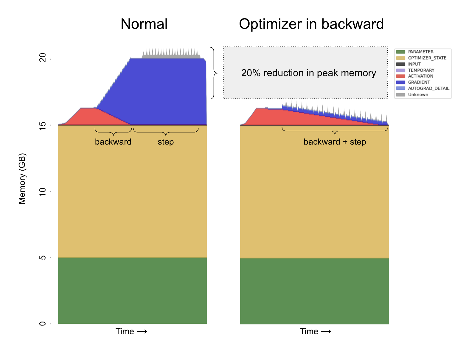
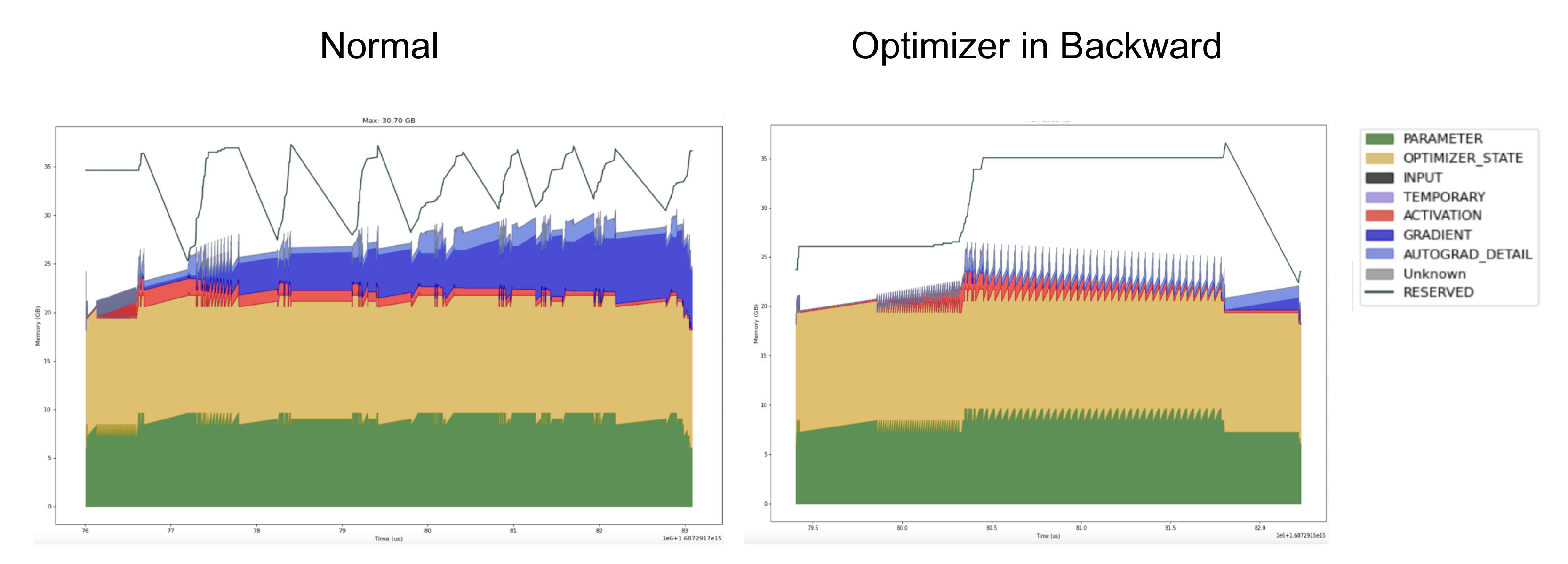
Normal PyTorch (left) and merged backward and optimizer (right). By applying the optimizer as soon as a gradient is computed we can immediately free each gradient and avoid storing all gradients for the backward pass. Example: stack of 20 Linear layers and AdamW. Simpler optimizers (e.g. SGD) will see an ever greater improvement (over 40% reduction.)
Real world example: Lit-LLaMA
Modern large language models have a voracious appetite for memory and will thrash long before they OOM. Performance will degrade and you’ll be left wondering what in your implementation is correct. Chances are, nothing is wrong: it’s just that your GPUs are under extreme memory pressure.
Here we show that by reducing memory pressure in the system we can obtain an 8.7x cost improvement in a real workload (pretraining Lit-LLaMA 7B https://github.com/lightning-AI/lit-llama) : a whopping 7x throughput improvement on 20% fewer GPUs.
Here’s what you need to do to leverage this optimization.
# import the new fsdp_overlap_step_with_backward context manager
from lightning.fabric.strategies.fsdp import fsdp_overlap_step_with_backward
# create one optimizer instance per parameter
optimizers = [Optimizer([p], ...) for p in model.parameters()]
...
for inputs, targets in epoch:
# run forward and compute the loss as usual
loss = loss_fn(model(inputs), targets)
# instead of calling optimizer.step(), call `loss.backward`
# within the fsdp_overlap_step_with_backward context, and the
# parameters will be automatically updated
with fsdp_overlap_step_with_backward(optimizers, model):
loss.backward()
This is all one needs to know to reap the benefits of this optimization.
However, the backstory is extremely interesting, so as a strictly optional reading, we’re happy to share the gnarly details as well as several other tricks.
Deep dive: Triaging and fixing a memory bound workload.
As mentioned above, we’ll be focusing on pre-training Lit-LLaMA 7B (https://github.com/lightning-AI/lit-llama), an open source implementation of the LLaMA model based on nanoGPT.
For this model we have about 24GB for the parameters, and 48 GB of AdamW state. We’ll start off by using FSDP to shard across 4 GPUs. You can find the pre-training code in this lit-llama branch (which adds extra instrumentation): https://github.com/Lightning-AI/lit-llama/tree/robieta/memory_blogpost.
Sadly, our training run will OOM shortly after starting on 4GPUs. Let’s dig deeper.
foreach and the surprising perils of fusion
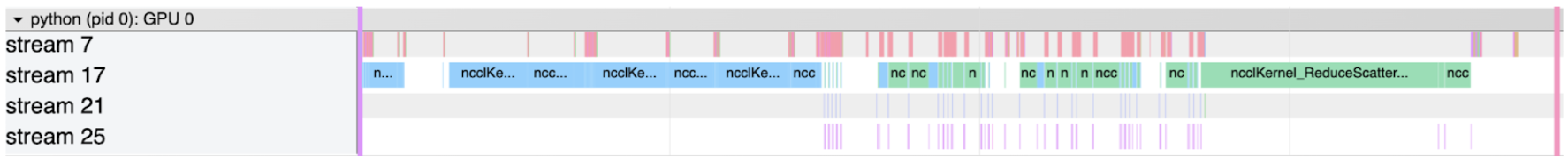
In order to get something running we’re going to briefly increase the number of GPUs from four to five. This will allow us to collect a profile and diagnose where we can save memory. It takes ~8 seconds to run, and a cursory glance at the GPU compute stream tells us our GPU utilization is extremely poor.
Each row on the table represents a GPU stream, which is where computations are executed one after the other. The compute streams (7, 21, and 25) are where kernels are executed. We can see a lot of gaps indicating an idle GPU, which is bad because we’re wasting time and money. Only the communication stream (17) shows high utilization, and as we’ll see later even that isn’t “real” saturation.
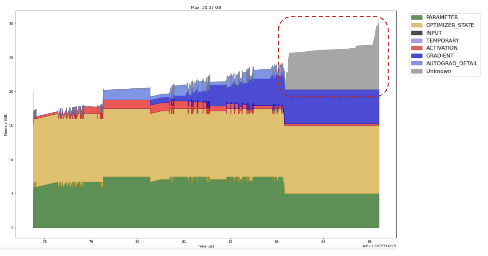
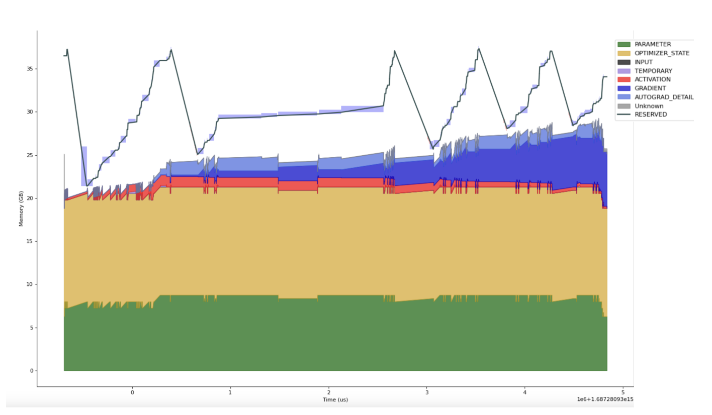
Taking a look at the memory profile for rank zero we see a large spike in memory utilization at the end of the step:
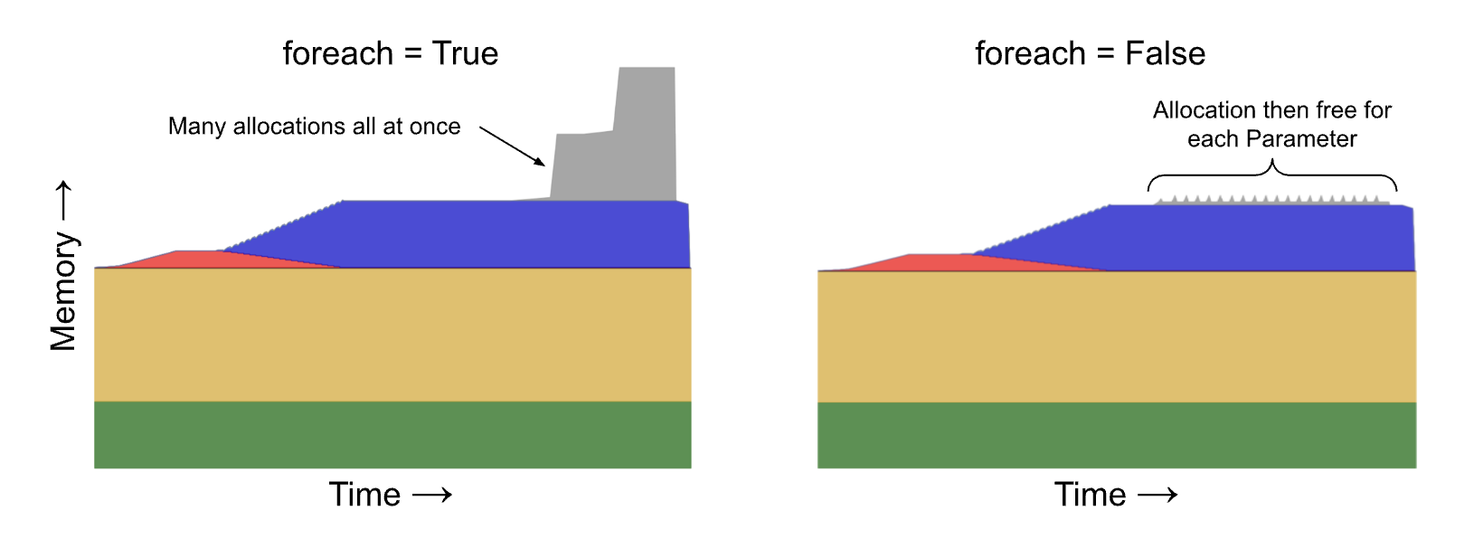
There’s an argument in PyTorch optimizers named foreach to group parameter updates. The idea is to amortize overhead by launching a small number of large operations rather than a large number of small kernels. See https://pytorch.org/docs/main/generated/torch.optim.AdamW.html as an example.
This argument defaults to True in AdamW. However this also means that rather than a sequence of “allocate, free, allocate, free, …” the grouping produces “allocate, allocate, …, free, free, …” which increases the peak memory from the optimizer from O(k) to O(n * k). (See this issue for a more detailed technical description.) In the initial figure we set foreach to a non-default value so as not to overly inflate the benefit of applying the optimizer during the backward pass.
Setting `foreach` to False reduces our step time to ~7.2 seconds. We’re now also able to run on 4 GPUs without running out of memory. Perplexingly however, 4 GPUs take virtually the same amount of time per step. We’ll see why in a moment.
Allocated vs. reserved memory
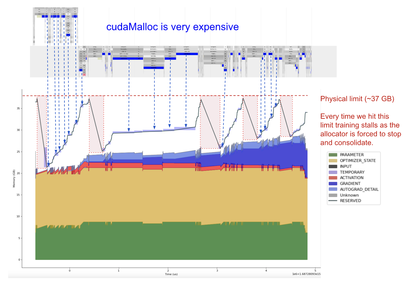
PyTorch uses a custom allocator called CUDACachingAllocator to allocate Tensor memory. The allocator itself is quite complicated. (Zach DeVito has an excellent blog post which gives an in-depth description.) Notably, the “Caching” part of “CUDACachingAllocator” refers to the fact that the allocator will hold onto a pool of memory blocks that it allocated from the CUDA runtime and try to reuse those to avoid expensive and synchronizing calls to cudaMalloc and cudaFree. This is why `nvidia-smi` generally reports higher memory consumption than torch.cuda.memory_allocated. If we overlay the total reserved memory on our memory profile we see that reserved memory is quite a bit higher than allocated memory. (The blue translucent blocks are cudaMalloc calls, which we’ll address in a moment.)
Every time the reserved memory reaches the limit of physical memory the system stalls as the CUDACachingAllocator is forced to stop and free unused reserved memory. The exact pattern for these spikes is non-deterministic and varies between ranks. The issue turns out to be communication: In order to overlap compute and communication FSDP aggressively enqueues all-reduce operations. However this also increases the amount of memory needed for the communication buffers backing these computations:
- These ops are also on a separate CUDA stream which is why we see non-determinism.
- The CUDACachingAllocator is not well suited to cache across streams due to some implementation details of how it exploits CUDA ordering.
Going back to the plot above, what we see is every time we reach the limit of physical memory there is a linear decrease in reserved memory as the allocator returns memory to the CUDA runtime, and then allocations immediately after these regions incur expensive cudaMalloc calls.
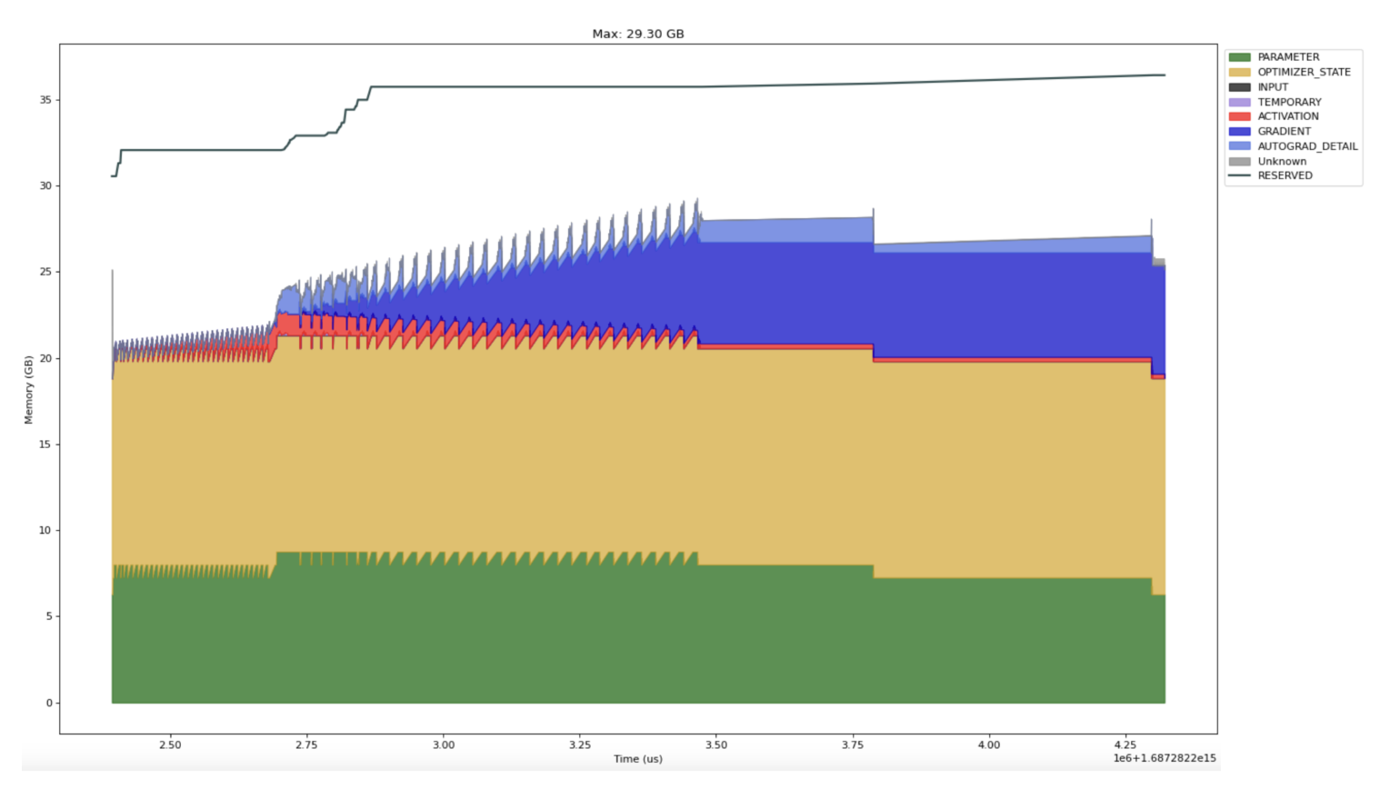
Fortunately FSDP has a flag to limit the number of all gathers. Setting `limit_all_gathers=True` cuts our step time down to 2.5 seconds. Reserved memory still hovers close to the limit, but we never reach the hard collection limit and there are no long calls to cudaMalloc or cudaFree. (Note that the effect is workload dependent. There have been several proposals to flip the default [1] [2] but as of writing none have been adopted.)
fsdp_overlap_step_with_backward
While our workload is much improved, there is still some memory pressure. Now that we’ve eliminated the most egregious sources we can turn our attention to the technique introduced in this blogpost: applying the optimizer step in the backward pass.
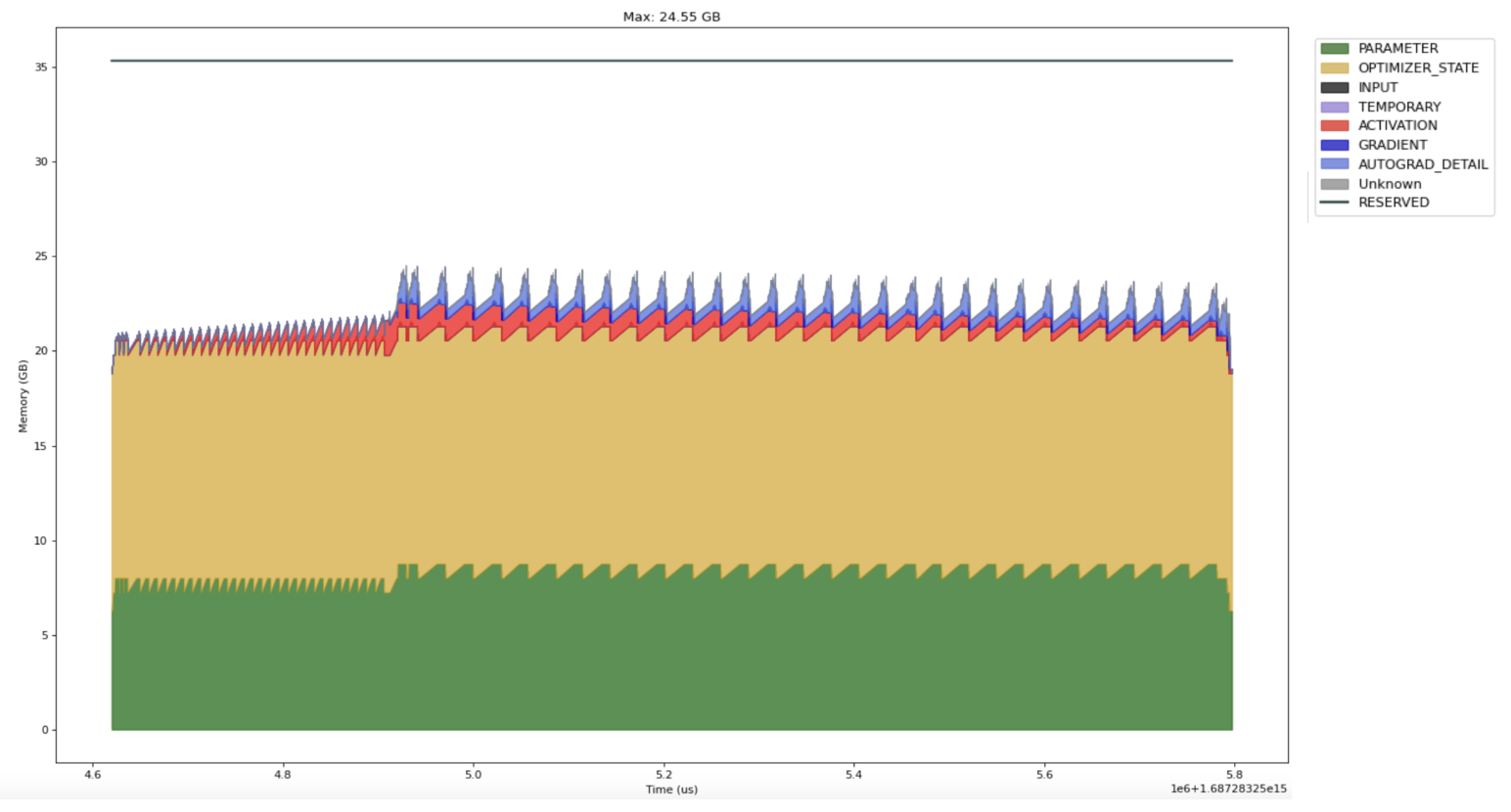
With this change our step time drops from ~2.5 seconds to ~1.15 seconds (!) and inspection of the timeline indicates that it is close to saturated. A 5 GB drop might not seem all that significant (particularly since our reserved memory hovers just under the limit), but we must recall the caching strategy employed by the CUDACachingAllocator: try to reuse blocks of similar size for subsequent allocations. This technique is much friendlier to that caching strategy because models tend to have repeated structure, so there is a high probability during the backward pass that recently freed blocks will be exactly the right size to satisfy new allocations. Consequently, we also see a 3.5x drop in the normalized standard deviation: 8% vs. 28% standard deviation of step time.
BackwardPrefetch.BACKWARD_POST: a compromise
There are a variety of knobs to reduce memory pressure. They tend to require tuning as they defer or recompute parts of the model in order to avoid storing values when memory pressure is highest. One such knob is prefetch timing: delaying prefetch allows us to consume less memory, but increases the likelihood of communication on the critical path. If we don’t combine backward and optimizer this flag reduces step time from 2.5 to 2.1 seconds. But if we do overlap them then it increases the step time from 1.15 to 1.25 seconds. Bear in mind that as memory pressure decreases certain optimizations can become pessimizations.
Scaling up: LLaMA 13B & 8 GPUs
Memory pressure on LLMs is a stochastic problem. This is due to the combination of multi-stream computation and complex heuristic runtime details. (such as the CUDACachingAllocator) as we scale up the straggler problem becomes more severe. To demonstrate this we’ll approximately double our model size and run it on 8 GPUs. Combined backward+optimizer runs in 2.6 seconds, while the conventional approach takes 8.8 seconds: a 3.4x difference compared to the 2.2x for 7B on 4 GPUs.
We can see that in the normal approach (left) reserved memory is jagged and there are frequent and varied stalls. By contrast, the optimizer+backward (right) approach is more regular (though not perfect) which helps it scale more efficiently.
Wrapping up
When training LLMs memory is both precious and easy to squander. Applying optimizer steps during the backward pass can deliver considerable memory and performance improvement and is rarely detrimental.