Key takeaway
Learn how to use gradient accumulation to train models with large batch sizes in order to work around hardware limitations when GPU memory is a concern.Previously, I shared an article using multi-GPU training strategies to speed up the finetuning of large language models. Several of these strategies include mechanisms such as model or tensor sharding that distributes the model weights and computations across different devices to work around GPU memory limitations.
However, many of us don’t have access to multi-GPU resources. This article therefore demonstrates a great workaround to train models with larger batch sizes when GPU memory is a concern: gradient accumulation.
Let’s Finetune BLOOM for Classification
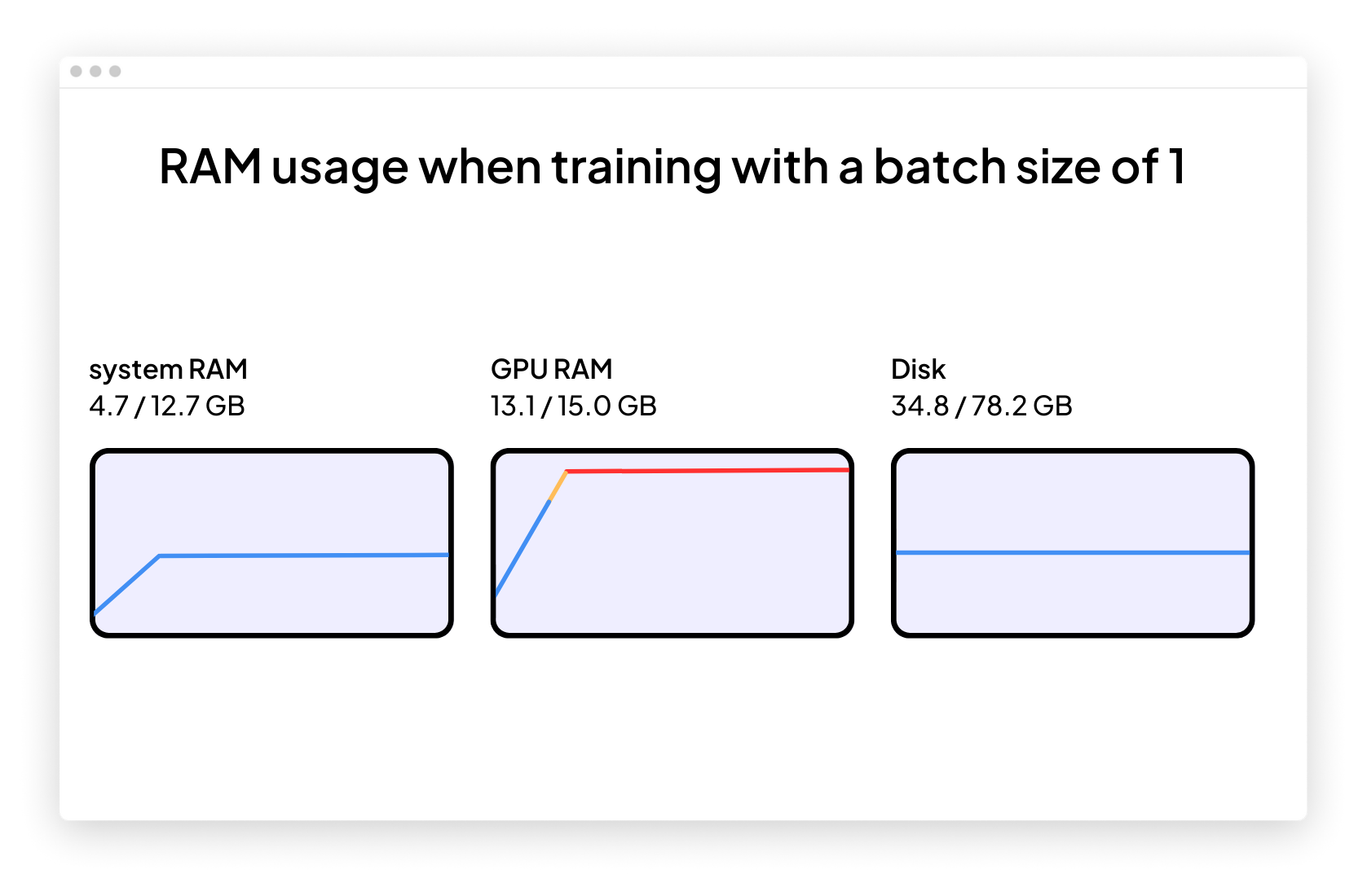
Let’s suppose we are interested in adopting a recent pretrained large language model for a downstream task such as text classification. We are going to work with BLOOM, which is an open-source alternative to GPT-3. In particular, we are going to use a version of BLOOM that “only” has 560 million parameters — it should fit into the RAM of conventional GPUs without problems (for reference, the free tier of Google Colab has a GPU with 15 Gb of RAM.)
Once we start, however, we bump into problems: our memory explodes during training or finetuning; we find that the only way to train this model is using a batch size of 1.
Note
The code for finetuning BLOOM for a target classification task using a batch size of 1 is shown below. (You can also download the complete code from GitHub here.)You can copy & paste this code directly into Google Colab. However, you also have to drag and drop the accompanying local_dataset_utilities.py file into the same folder as we import some dataset utilities from this file.
# pip install torch lightning matplotlib pandas torchmetrics watermark transformers datasets -U
import os
import os.path as op
import time
from datasets import load_dataset
from lightning import Fabric
import torch
from torch.utils.data import DataLoader
import torchmetrics
from transformers import AutoTokenizer
from transformers import AutoModelForSequenceClassification
from watermark import watermark
from local_dataset_utilities import download_dataset, load_dataset_into_to_dataframe, partition_dataset
from local_dataset_utilities import IMDBDataset
def tokenize_text(batch):
return tokenizer(batch["text"], truncation=True, padding=True, max_length=1024)
def train(num_epochs, model, optimizer, train_loader, val_loader, fabric):
for epoch in range(num_epochs):
train_acc = torchmetrics.Accuracy(
task="multiclass", num_classes=2).to(fabric.device)
for batch_idx, batch in enumerate(train_loader):
model.train()
### FORWARD AND BACK PROP
outputs = model(
batch["input_ids"],
attention_mask=batch["attention_mask"],
labels=batch["label"]
)
fabric.backward(outputs["loss"])
### UPDATE MODEL PARAMETERS
optimizer.step()
optimizer.zero_grad()
### LOGGING
if not batch_idx % 300:
print(f"Epoch: {epoch+1:04d}/{num_epochs:04d} "
f"| Batch {batch_idx:04d}/{len(train_loader):04d} "
f"| Loss: {outputs['loss']:.4f}")
model.eval()
with torch.no_grad():
predicted_labels = torch.argmax(outputs["logits"], 1)
train_acc.update(predicted_labels, batch["label"])
### MORE LOGGING
model.eval()
with torch.no_grad():
val_acc = torchmetrics.Accuracy(task="multiclass", num_classes=2).to(fabric.device)
for batch in val_loader:
outputs = model(
batch["input_ids"],
attention_mask=batch["attention_mask"],
labels=batch["label"]
)
predicted_labels = torch.argmax(outputs["logits"], 1)
val_acc.update(predicted_labels, batch["label"])
print(f"Epoch: {epoch+1:04d}/{num_epochs:04d} "
f"| Train acc.: {train_acc.compute()*100:.2f}% "
f"| Val acc.: {val_acc.compute()*100:.2f}%"
)
train_acc.reset(), val_acc.reset()
if __name__ == "__main__":
print(watermark(packages="torch,lightning,transformers", python=True))
print("Torch CUDA available?", torch.cuda.is_available())
device = "cuda" if torch.cuda.is_available() else "cpu"
torch.manual_seed(123)
# torch.use_deterministic_algorithms(True)
##########################
### 1 Loading the Dataset
##########################
download_dataset()
df = load_dataset_into_to_dataframe()
if not (op.exists("train.csv") and op.exists("val.csv") and op.exists("test.csv")):
partition_dataset(df)
imdb_dataset = load_dataset(
"csv",
data_files={
"train": "train.csv",
"validation": "val.csv",
"test": "test.csv",
},
)
#########################################
### 2 Tokenization and Numericalization
#########################################
tokenizer = AutoTokenizer.from_pretrained("bigscience/bloom-560m", max_length=1024)
print("Tokenizer input max length:", tokenizer.model_max_length, flush=True)
print("Tokenizer vocabulary size:", tokenizer.vocab_size, flush=True)
print("Tokenizing ...", flush=True)
imdb_tokenized = imdb_dataset.map(tokenize_text, batched=True, batch_size=None)
del imdb_dataset
imdb_tokenized.set_format("torch", columns=["input_ids", "attention_mask", "label"])
os.environ["TOKENIZERS_PARALLELISM"] = "false"
#########################################
### 3 Set Up DataLoaders
#########################################
train_dataset = IMDBDataset(imdb_tokenized, partition_key="train")
val_dataset = IMDBDataset(imdb_tokenized, partition_key="validation")
test_dataset = IMDBDataset(imdb_tokenized, partition_key="test")
train_loader = DataLoader(
dataset=train_dataset,
batch_size=1,
shuffle=True,
num_workers=4,
drop_last=True,
)
val_loader = DataLoader(
dataset=val_dataset,
batch_size=1,
num_workers=4,
drop_last=True,
)
test_loader = DataLoader(
dataset=test_dataset,
batch_size=1,
num_workers=2,
drop_last=True,
)
#########################################
### 4 Initializing the Model
#########################################
fabric = Fabric(accelerator="cuda", devices=1, precision="16-mixed")
fabric.launch()
model = AutoModelForSequenceClassification.from_pretrained(
"bigscience/bloom-560m", num_labels=2)
optimizer = torch.optim.Adam(model.parameters(), lr=5e-5)
model, optimizer = fabric.setup(model, optimizer)
train_loader, val_loader, test_loader = fabric.setup_dataloaders(
train_loader, val_loader, test_loader)
#########################################
### 5 Finetuning
#########################################
start = time.time()
train(
num_epochs=1,
model=model,
optimizer=optimizer,
train_loader=train_loader,
val_loader=val_loader,
fabric=fabric,
)
end = time.time()
elapsed = end-start
print(f"Time elapsed {elapsed/60:.2f} min")
with torch.no_grad():
model.eval()
test_acc = torchmetrics.Accuracy(task="multiclass", num_classes=2).to(fabric.device)
for batch in test_loader:
outputs = model(
batch["input_ids"],
attention_mask=batch["attention_mask"],
labels=batch["label"]
)
predicted_labels = torch.argmax(outputs["logits"], 1)
test_acc.update(predicted_labels, batch["label"])
print(f"Test accuracy {test_acc.compute()*100:.2f}%")
I am using Lightning Fabric because it allows me to flexibly change the number of GPUs and multi-GPU training strategy when running this code on different hardware. It also lets me enable mixed-precision training by only adjusting the precision flag. In this case, mixed-precision training can triple the training speed and reduce memory requirements by roughly 25%.
The main code shown above is executed in the if __name__ == "__main__" context, which is recommended when running Python scripts for multi-GPU training with PyTorch — even though we are only using a single GPU, it’s a best practice that we adopt. Then, the following three code sections within the if __name__ == "__main__", take care of the data loading:
# 1 Loading the Dataset
# 2 Tokenization and Numericalization
# 3 Setting Up DataLoaders
In section # 4 Initializing the Model, we initialize the model. Then, in section # 5 Finetuning, we call the train function, which is where things get interesting. In the train(...) function, we implement our standard PyTorch loop. An annotated version of the core training loop is shown below.
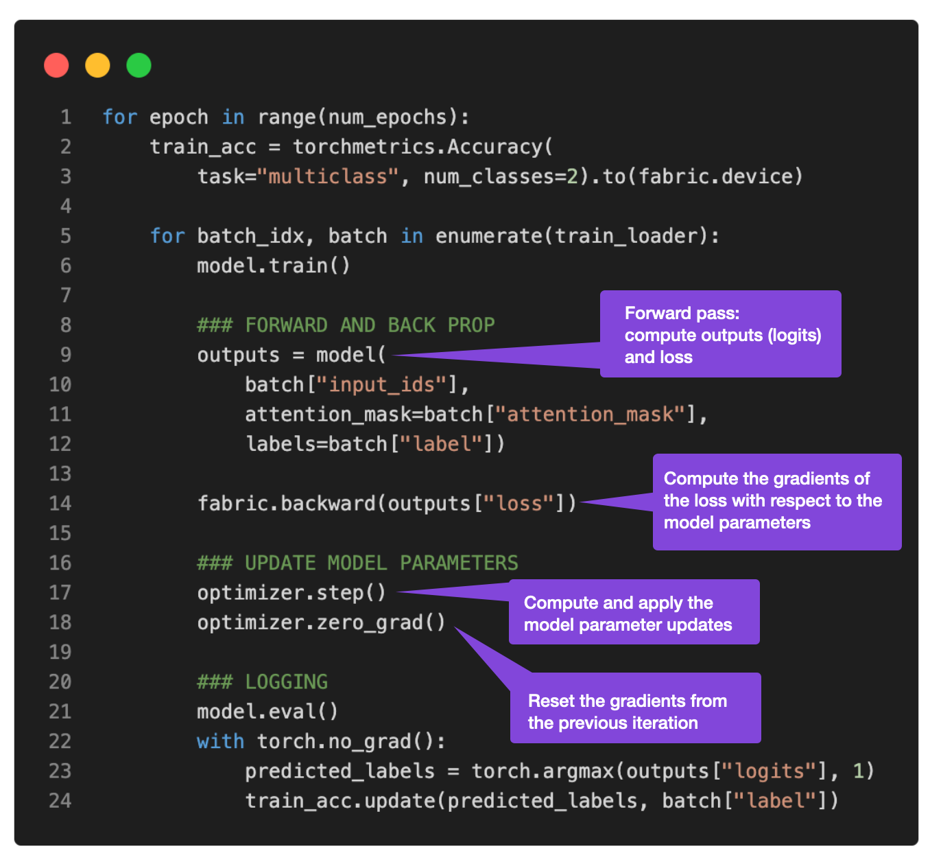
The problem with batch sizes of 1 is that the gradient updates will be extremely noisy, as we can see based on the fluctuating training loss and poor test set performance below when we train the model:
...
torch : 2.0.0
lightning : 2.0.0
transformers: 4.27.2
Torch CUDA available? True
...
Epoch: 0001/0001 | Batch 23700/35000 | Loss: 0.0969
Epoch: 0001/0001 | Batch 24000/35000 | Loss: 1.9902
Epoch: 0001/0001 | Batch 24300/35000 | Loss: 0.0395
Epoch: 0001/0001 | Batch 24600/35000 | Loss: 0.2546
Epoch: 0001/0001 | Batch 24900/35000 | Loss: 0.1128
Epoch: 0001/0001 | Batch 25200/35000 | Loss: 0.2661
Epoch: 0001/0001 | Batch 25500/35000 | Loss: 0.0044
Epoch: 0001/0001 | Batch 25800/35000 | Loss: 0.0067
Epoch: 0001/0001 | Batch 26100/35000 | Loss: 0.0468
Epoch: 0001/0001 | Batch 26400/35000 | Loss: 1.7139
Epoch: 0001/0001 | Batch 26700/35000 | Loss: 0.9570
Epoch: 0001/0001 | Batch 27000/35000 | Loss: 0.1857
Epoch: 0001/0001 | Batch 27300/35000 | Loss: 0.0090
Epoch: 0001/0001 | Batch 27600/35000 | Loss: 0.9790
Epoch: 0001/0001 | Batch 27900/35000 | Loss: 0.0503
Epoch: 0001/0001 | Batch 28200/35000 | Loss: 0.2625
Epoch: 0001/0001 | Batch 28500/35000 | Loss: 0.1010
Epoch: 0001/0001 | Batch 28800/35000 | Loss: 0.0035
Epoch: 0001/0001 | Batch 29100/35000 | Loss: 0.0009
Epoch: 0001/0001 | Batch 29400/35000 | Loss: 0.0234
Epoch: 0001/0001 | Batch 29700/35000 | Loss: 0.8394
Epoch: 0001/0001 | Batch 30000/35000 | Loss: 0.9497
Epoch: 0001/0001 | Batch 30300/35000 | Loss: 0.1437
Epoch: 0001/0001 | Batch 30600/35000 | Loss: 0.1317
Epoch: 0001/0001 | Batch 30900/35000 | Loss: 0.0112
Epoch: 0001/0001 | Batch 31200/35000 | Loss: 0.0073
Epoch: 0001/0001 | Batch 31500/35000 | Loss: 0.7393
Epoch: 0001/0001 | Batch 31800/35000 | Loss: 0.0512
Epoch: 0001/0001 | Batch 32100/35000 | Loss: 0.1337
Epoch: 0001/0001 | Batch 32400/35000 | Loss: 1.1875
Epoch: 0001/0001 | Batch 32700/35000 | Loss: 0.2727
Epoch: 0001/0001 | Batch 33000/35000 | Loss: 0.1545
Epoch: 0001/0001 | Batch 33300/35000 | Loss: 0.0022
Epoch: 0001/0001 | Batch 33600/35000 | Loss: 0.2681
Epoch: 0001/0001 | Batch 33900/35000 | Loss: 0.2467
Epoch: 0001/0001 | Batch 34200/35000 | Loss: 0.0620
Epoch: 0001/0001 | Batch 34500/35000 | Loss: 2.5039
Epoch: 0001/0001 | Batch 34800/35000 | Loss: 0.0131
Epoch: 0001/0001 | Train acc.: 75.11% | Val acc.: 78.62%
Time elapsed 69.97 min
Test accuracy 78.53%
Since we don’t have multiple GPUs available for tensor sharding, what can we do to train the model with larger batch sizes?
One workaround is gradient accumulation, where we modify the aforementioned training loop.
What is gradient accumulation?
Gradient accumulation is a way to virtually increase the batch size during training, which is very useful when the available GPU memory is insufficient to accommodate the desired batch size. In gradient accumulation, gradients are computed for smaller batches and accumulated (usually summed or averaged) over multiple iterations instead of updating the model weights after every batch. Once the accumulated gradients reach the target “virtual” batch size, the model weights are updated with the accumulated gradients.To illustrate this, consider the updated PyTorch training loop below. (The full script is available here on GitHub.)
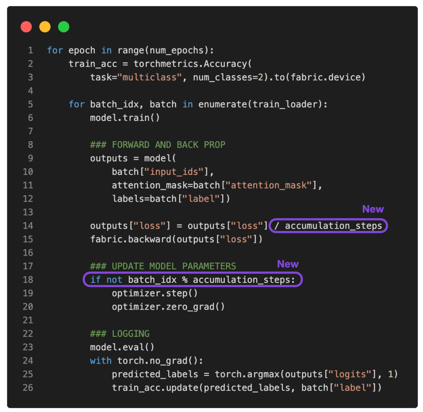
If we set accumulation_steps to 2, then zero_grad() and optimizer.step() will only be called every second epoch. Consequently, running the modified training loop with accumulation_steps=2 will have the same effect as doubling the batch size.
For example, if we want to use a batch size of 256 but can only fit a batch size of 64 into GPU memory, we can perform gradient accumulation over four batches of size 64. (After processing all four batches, we will have the accumulated gradients equivalent to a single batch of size 256.) This allows us to effectively emulate a larger batch size without requiring larger GPU memory or tensor sharding across different devices.
While gradient accumulation can help us train models with larger batch sizes, it does not reduce the total computation required. In fact, it can sometimes lead to a slightly slower training process, as the weight updates are performed less frequently. Nevertheless, it allows us to work around limitations where we have very small batch sizes that lead to noisy updates.
For example, let’s now run the code from above, where we have a batch size of 1, with 16 accumulation steps to simulate a batch size of 16. You can download the code here.
The output is as follows:
...
torch : 2.0.0
lightning : 2.0.0
transformers: 4.27.2
Torch CUDA available? True
...
Epoch: 0001/0001 | Batch 23700/35000 | Loss: 0.0168
Epoch: 0001/0001 | Batch 24000/35000 | Loss: 0.0006
Epoch: 0001/0001 | Batch 24300/35000 | Loss: 0.0152
Epoch: 0001/0001 | Batch 24600/35000 | Loss: 0.0003
Epoch: 0001/0001 | Batch 24900/35000 | Loss: 0.0623
Epoch: 0001/0001 | Batch 25200/35000 | Loss: 0.0010
Epoch: 0001/0001 | Batch 25500/35000 | Loss: 0.0001
Epoch: 0001/0001 | Batch 25800/35000 | Loss: 0.0047
Epoch: 0001/0001 | Batch 26100/35000 | Loss: 0.0004
Epoch: 0001/0001 | Batch 26400/35000 | Loss: 0.1016
Epoch: 0001/0001 | Batch 26700/35000 | Loss: 0.0021
Epoch: 0001/0001 | Batch 27000/35000 | Loss: 0.0015
Epoch: 0001/0001 | Batch 27300/35000 | Loss: 0.0008
Epoch: 0001/0001 | Batch 27600/35000 | Loss: 0.0060
Epoch: 0001/0001 | Batch 27900/35000 | Loss: 0.0001
Epoch: 0001/0001 | Batch 28200/35000 | Loss: 0.0426
Epoch: 0001/0001 | Batch 28500/35000 | Loss: 0.0012
Epoch: 0001/0001 | Batch 28800/35000 | Loss: 0.0025
Epoch: 0001/0001 | Batch 29100/35000 | Loss: 0.0025
Epoch: 0001/0001 | Batch 29400/35000 | Loss: 0.0000
Epoch: 0001/0001 | Batch 29700/35000 | Loss: 0.0495
Epoch: 0001/0001 | Batch 30000/35000 | Loss: 0.0164
Epoch: 0001/0001 | Batch 30300/35000 | Loss: 0.0067
Epoch: 0001/0001 | Batch 30600/35000 | Loss: 0.0037
Epoch: 0001/0001 | Batch 30900/35000 | Loss: 0.0005
Epoch: 0001/0001 | Batch 31200/35000 | Loss: 0.0013
Epoch: 0001/0001 | Batch 31500/35000 | Loss: 0.0112
Epoch: 0001/0001 | Batch 31800/35000 | Loss: 0.0053
Epoch: 0001/0001 | Batch 32100/35000 | Loss: 0.0012
Epoch: 0001/0001 | Batch 32400/35000 | Loss: 0.1365
Epoch: 0001/0001 | Batch 32700/35000 | Loss: 0.0210
Epoch: 0001/0001 | Batch 33000/35000 | Loss: 0.0374
Epoch: 0001/0001 | Batch 33300/35000 | Loss: 0.0007
Epoch: 0001/0001 | Batch 33600/35000 | Loss: 0.0341
Epoch: 0001/0001 | Batch 33900/35000 | Loss: 0.0259
Epoch: 0001/0001 | Batch 34200/35000 | Loss: 0.0005
Epoch: 0001/0001 | Batch 34500/35000 | Loss: 0.4792
Epoch: 0001/0001 | Batch 34800/35000 | Loss: 0.0003
Epoch: 0001/0001 | Train acc.: 78.67% | Val acc.: 87.28%
Time elapsed 51.37 min
Test accuracy 87.37%
As we can see, based on the results above, the loss fluctuates less than before. In addition, the test set performance increased by 10%! We are only iterating through the training set once, so each training example is only encountered a single time. Training the model for multiple epochs can further improve the predictive performance, but I’ll leave this as an exercise for you to try out (and let me know how it goes on Discord!).
You may have also noticed that this code also executed faster than the code we used previously with a batch size of 1. If we increase the virtual batch size to 8 using gradient accumulation, we still have the same number of forward passes. However, since we only update the model every eighth epoch, we have fewer backward passes, which lets us iterate through the examples in a single epoch faster.
Conclusion
Gradient accumulation is a technique that simulates a larger batch size by accumulating gradients from multiple small batches before performing a weight update. This technique can be helpful in scenarios where the available memory is limited, and the batch size that can fit in memory is small.
However, consider a scenario in which you can run the batch size in the first place, meaning the available memory is large enough to accommodate the desired batch size. In that case, gradient accumulation may not be necessary. In fact, running a larger batch size can be more efficient because it allows for more parallelism and reduces the number of weight updates required to train the model.
In summary, gradient accumulation can be a useful technique for reducing the impact of noise in small batch sizes on the accuracy of gradient updates. It’s a simple yet effective technique that lets us work around hardware limitations.
For reference, all code accompanying this blog post is available here on GitHub.
PS: Can we make this run even faster?
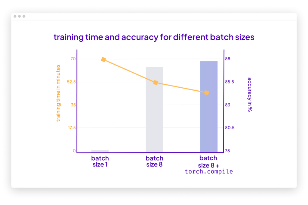
Yes! We can make it run even faster using torch.compile introduced in PyTorch 2.0. All it takes is a little addition of model = torch.compile, as shown in the figure below.
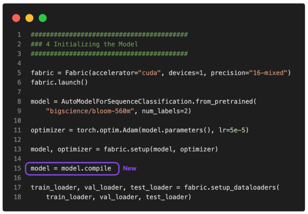 The full script is available on GitHub.
In this case, torch.compile shaves off another ten minutes of training without impacting the modeling performance:
poch: 0001/0001 | Batch 26400/35000 | Loss: 0.0320
Epoch: 0001/0001 | Batch 26700/35000 | Loss: 0.0010
Epoch: 0001/0001 | Batch 27000/35000 | Loss: 0.0006
Epoch: 0001/0001 | Batch 27300/35000 | Loss: 0.0015
Epoch: 0001/0001 | Batch 27600/35000 | Loss: 0.0157
Epoch: 0001/0001 | Batch 27900/35000 | Loss: 0.0015
Epoch: 0001/0001 | Batch 28200/35000 | Loss: 0.0540
Epoch: 0001/0001 | Batch 28500/35000 | Loss: 0.0035
Epoch: 0001/0001 | Batch 28800/35000 | Loss: 0.0016
Epoch: 0001/0001 | Batch 29100/35000 | Loss: 0.0015
Epoch: 0001/0001 | Batch 29400/35000 | Loss: 0.0008
Epoch: 0001/0001 | Batch 29700/35000 | Loss: 0.0877
Epoch: 0001/0001 | Batch 30000/35000 | Loss: 0.0232
Epoch: 0001/0001 | Batch 30300/35000 | Loss: 0.0014
Epoch: 0001/0001 | Batch 30600/35000 | Loss: 0.0032
Epoch: 0001/0001 | Batch 30900/35000 | Loss: 0.0004
Epoch: 0001/0001 | Batch 31200/35000 | Loss: 0.0062
Epoch: 0001/0001 | Batch 31500/35000 | Loss: 0.0032
Epoch: 0001/0001 | Batch 31800/35000 | Loss: 0.0066
Epoch: 0001/0001 | Batch 32100/35000 | Loss: 0.0017
Epoch: 0001/0001 | Batch 32400/35000 | Loss: 0.1485
Epoch: 0001/0001 | Batch 32700/35000 | Loss: 0.0324
Epoch: 0001/0001 | Batch 33000/35000 | Loss: 0.0155
Epoch: 0001/0001 | Batch 33300/35000 | Loss: 0.0007
Epoch: 0001/0001 | Batch 33600/35000 | Loss: 0.0049
Epoch: 0001/0001 | Batch 33900/35000 | Loss: 0.1170
Epoch: 0001/0001 | Batch 34200/35000 | Loss: 0.0002
Epoch: 0001/0001 | Batch 34500/35000 | Loss: 0.4201
Epoch: 0001/0001 | Batch 34800/35000 | Loss: 0.0018
Epoch: 0001/0001 | Train acc.: 78.39% | Val acc.: 86.84%
Time elapsed 43.33 min
Test accuracy 87.91%
Note that the slight accuracy improvement compared to before is likely due to randomness.