Tensor Parallelism
Tensor parallelism is a technique for training large models by distributing layers across multiple devices, improving memory management and efficiency by reducing inter-device communication. However, for smaller models, the communication overhead may outweigh its benefits. This method is most effective for models with very large layers, significantly enhancing performance and memory efficiency.
How to exploit parallelism in linear layers
In tensor parallelism, the computation of a linear layer can be split up across GPUs. This saves memory because each GPU only needs to hold a portion of the weight matrix. There are two ways a linear layer can be split up: row-wise or column-wise.
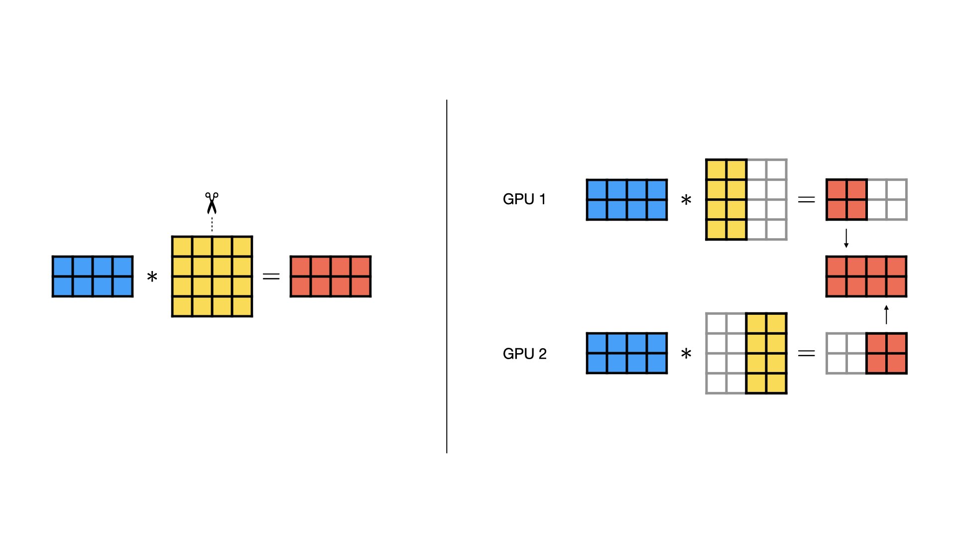
Column-wise Parallel
In a column-wise parallel layer, the weight matrix is split evenly along the column dimension. Each GPU is sent the same input, and computes a regular matrix multiplication with its portion of the weight matrix. At the end, the outputs from each GPU can be concatenated to form the final output.

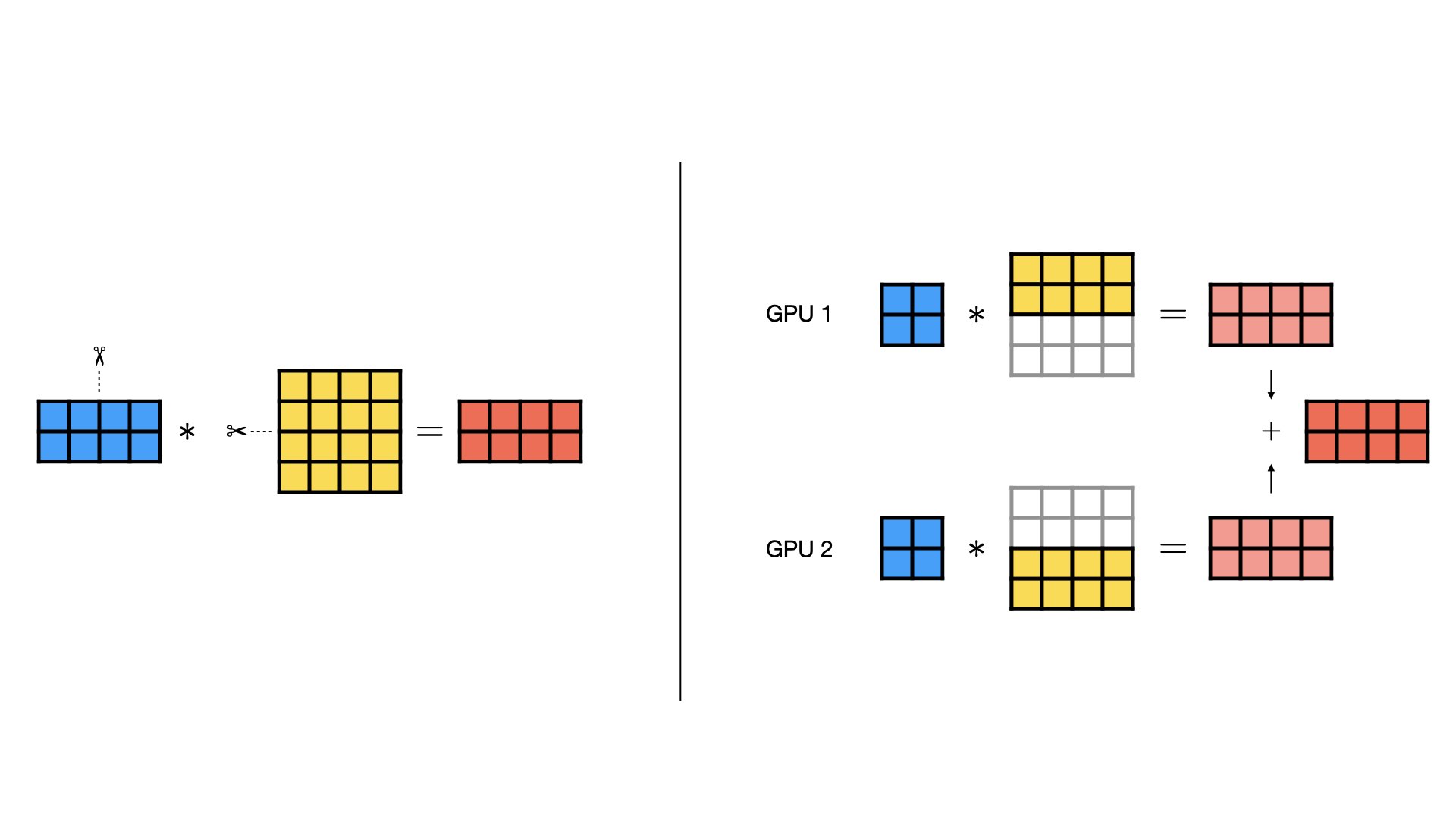
Row-wise Parallel
Row-wise parallelism divides the rows of the weight matrix evenly across devices. In addition, the input gets split the same way along the inner dimension (because the weight matrix now has fewer rows). Each GPU then performs a regular matrix multiplication with its portion of the weight matrix and inputs. At the end, the outputs from each GPU can be summed up element-wise (all-reduce) to form the final output.

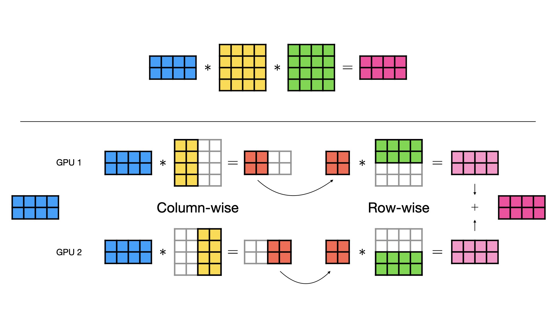
Combined Column- and Row-wise Parallel
When there are multiple linear layers in sequence, e.g., in a MLP or a Transformer, the column-wise and row-wise parallel styles can be combined for maximum effect. Instead of concatenating the output of the column-wise parallel layer, we keep the outputs separate and feed them directly to the row-wise parallel layer. This way, we avoid costly data transfers between GPUs.

Note that activation functions between the layers can still be applied without additional communication because they are element-wise, but are not shown in the figures for simplicity.
Apply tensor parallelism to a model
To apply tensor parallelism to a model with Fabric, you need a good understanding of your model’s architecture to make the decision of where to apply the parallel styles you’ve seen above. Let’s start with a simple MLP toy example:
import torch.nn as nn
import torch.nn.functional as F


class FeedForward(nn.Module):
    def __init__(self, dim, hidden_dim):
        super().__init__()
        self.w1 = nn.Linear(dim, hidden_dim, bias=False)
        self.w2 = nn.Linear(hidden_dim, dim, bias=False)
        self.w3 = nn.Linear(dim, hidden_dim, bias=False)

    def forward(self, x):
        return self.w2(F.silu(self.w1(x)) * self.w3(x))
This model has three linear layers. Layers w1 and w3 produce an output that is later multiplied element-wise.
That output is then fed into layer w2.
Therefore, w1 and w3 are suitable candidates for column-wise parallelism, because their output(s) can easily be combined with w2 in row-wise fashion.
In Fabric, define a function that applies the tensor parallelism to the model:
from torch.distributed.tensor.parallel import ColwiseParallel, RowwiseParallel
from torch.distributed.tensor.parallel import parallelize_module


def parallelize_feedforward(model, device_mesh):
    # Lightning will set up a device mesh for you
    tp_mesh = device_mesh["tensor_parallel"]
    # Use PyTorch's distributed tensor APIs to parallelize the model
    plan = {
        "w1": ColwiseParallel(),
        "w2": RowwiseParallel(),
        "w3": ColwiseParallel(),
    }
    parallelize_module(model, tp_mesh, plan)
    return model
By writing the parallelization code in a separate function rather than hardcoding it into the model, we keep the original source code clean and maintainable.
Next, configure the ModelParallelStrategy in Fabric:
import lightning as L
from lightning.fabric.strategies import ModelParallelStrategy

# 1. Pass the parallelization function to the strategy
strategy = ModelParallelStrategy(parallelize_fn=parallelize_feedforward)

# 2. Configure devices and set the strategy in Fabric
fabric = L.Fabric(accelerator="cuda", devices=2, strategy=strategy)
fabric.launch()
The strategy takes the custom parallelization function as input.
No other changes to your training code are necessary at this point.
Later in the code, when you call fabric.setup(model), Fabric will apply the parallelize_feedforward function to the model automatically.
Full training example (requires at least 2 GPUs).
import torch
import torch.nn as nn
import torch.nn.functional as F

from torch.distributed.tensor.parallel import ColwiseParallel, RowwiseParallel
from torch.distributed.tensor.parallel import parallelize_module

import lightning as L
from lightning.pytorch.demos.boring_classes import RandomDataset
from lightning.fabric.strategies import ModelParallelStrategy


class FeedForward(nn.Module):
    def __init__(self, dim, hidden_dim):
        super().__init__()
        self.w1 = nn.Linear(dim, hidden_dim, bias=False)
        self.w2 = nn.Linear(hidden_dim, dim, bias=False)
        self.w3 = nn.Linear(dim, hidden_dim, bias=False)

    def forward(self, x):
        return self.w2(F.silu(self.w1(x)) * self.w3(x))


def parallelize_feedforward(model, device_mesh):
    # Lightning will set up a device mesh for you
    tp_mesh = device_mesh["tensor_parallel"]
    # Use PyTorch's distributed tensor APIs to parallelize the model
    plan = {
        "w1": ColwiseParallel(),
        "w2": RowwiseParallel(),
        "w3": ColwiseParallel(),
    }
    parallelize_module(model, tp_mesh, plan)
    return model


strategy = ModelParallelStrategy(parallelize_fn=parallelize_feedforward)
fabric = L.Fabric(accelerator="cuda", devices=2, strategy=strategy)
fabric.launch()

# Initialize the model
model = FeedForward(8192, 8192)
model = fabric.setup(model)

# Define the optimizer
optimizer = torch.optim.AdamW(model.parameters(), lr=3e-3)
optimizer = fabric.setup_optimizers(optimizer)

# Define dataset/dataloader
dataset = RandomDataset(8192, 64)
dataloader = torch.utils.data.DataLoader(dataset, batch_size=8)
dataloader = fabric.setup_dataloaders(dataloader)

# Simplified training loop
for i, batch in enumerate(dataloader):
    output = model(batch)
    loss = output.sum()
    fabric.backward(loss)
    optimizer.step()
    optimizer.zero_grad()
    fabric.print(f"Iteration {i} complete")

fabric.print(f"Peak memory usage: {torch.cuda.max_memory_allocated() / 1e9:.02f} GB")
Note
Tensor Parallelism in Lightning Fabric as well as PyTorch is experimental. The APIs may change in the future.
When measuring the peak memory consumption, we should see that doubling the number of GPUs reduces the memory consumption roughly by half:
1 GPU (no TP) |
2 GPUs |
4 GPUs |
8 GPUs |
|
|---|---|---|---|---|
Memory per GPU |
4.04 GB |
2.03 GB |
1.02 GB |
0.60 GB |
Beyond this toy example, we recommend you study our LLM Tensor Parallel Example (Llama 3).
Data-loading considerations
In a tensor-parallelized model, it is important that the model receives an identical input on each GPU. Otherwise, training won’t converge. Therefore, when you shuffle data in your dataset or data loader, or when applying randomized transformations/augmentations in your data, ensure that the seed is set appropriately.
Given this requirement, your global batch size will be limited by the memory of a single GPU. To scale the batch size and accelerate training further, you can combine tensor parallelism with data parallelism (in particular, FSDP).
